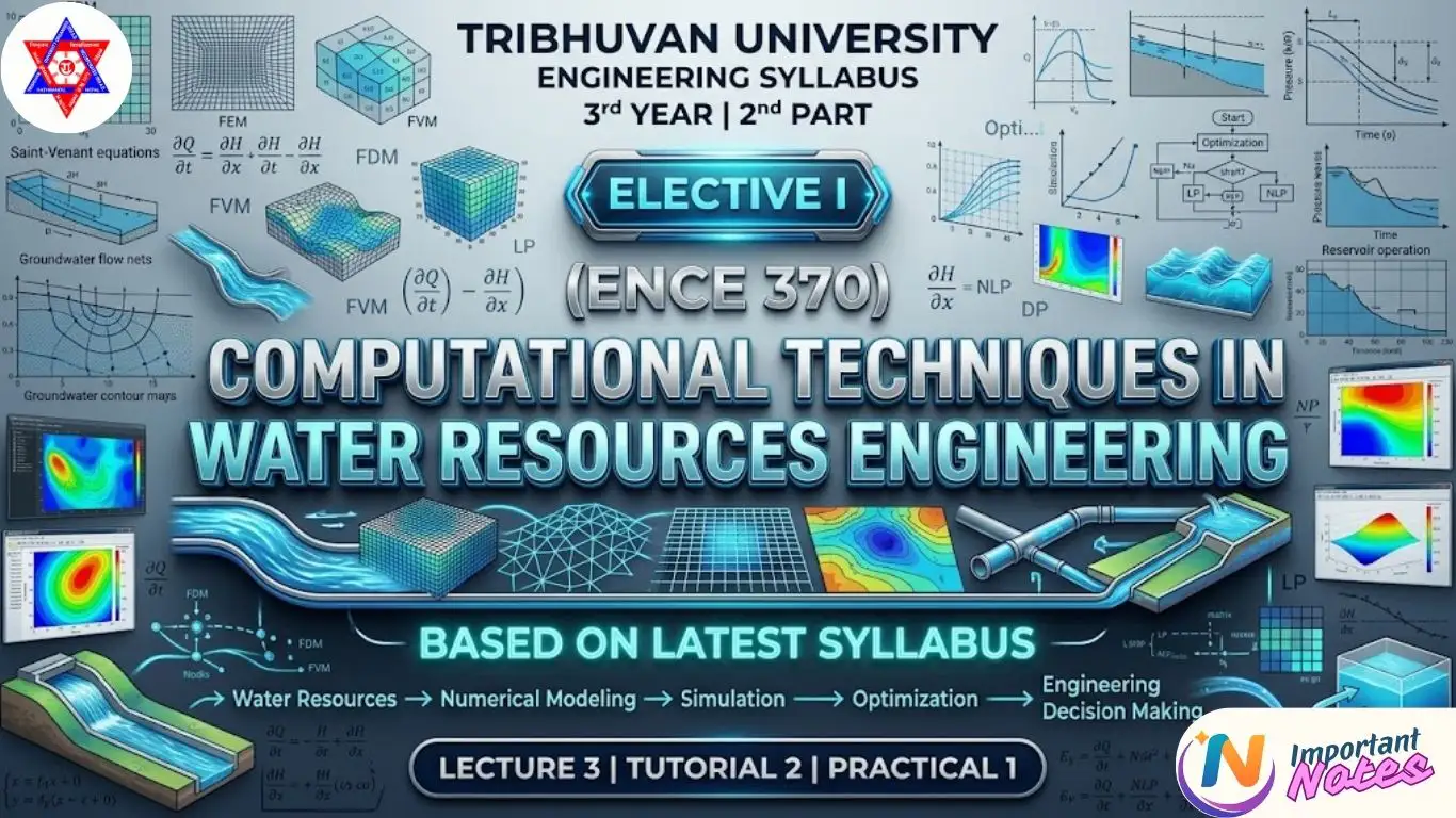
Computational Techniques in Water Resources Engineering: Chapter 1 Notes

Fundamentals of Computational Techniques in Water Resources

Water resources engineering deals with physical phenomena governing open channel flows, groundwater transport, pipe network hydraulics, and atmospheric precipitation. Because closed-form mathematical solutions are restricted to highly simplified geometry and steady flow states, modern civil engineers rely on computational techniques in water resources to perform hydrodynamic simulations under unsteady, non-uniform, and multi-dimensional real-world conditions.

1. Role of Computational Techniques in Water Resources Management

The primary objectives of employing numerical computations in hydraulic engineering include:

• Flood Wave Routing & Inundation Mapping: Simulating dam breaks, river surcharges, and coastal storm surges to issue timely warnings and construct flood mitigation infrastructure.
• Groundwater & Aquifer Management: Predicting drawdown, contaminant plume migration, and saltwater intrusion using differential flow equations.
• Urban Drainage Infrastructure Design: Sizing storm sewers, retention basins, and culverts under dynamic rainfall-runoff conditions.
• Sediment & Pollution Transport Modeling: Simulating bed level changes, scour around bridge piers, and water quality kinetics in lakes and estuaries.

2. Classification of Water Resources Models

Hydro-environmental models fall into three broad mathematical categories:

A. Deterministic Models

Deterministic models operate on physical conservation laws (conservation of mass, momentum, and energy) without incorporating random variation. For a given set of input parameters and initial states, a deterministic model will always yield the exact same output. Examples include Saint-Venant hydrodynamic routing and Navier-Stokes hydraulic models.

B. Stochastic Models

Stochastic models account for inherent randomness and uncertainty in natural hydrological systems. They represent variables using probability distributions rather than fixed single values. Examples include autoregressive moving average (ARMA) time series models for annual streamflow generation and Monte Carlo rainfall simulations.

C. Data-Driven Models

Data-driven models bypass explicit physical conservation formulations by extracting complex non-linear relationships directly from historical monitoring data. Examples include Artificial Neural Networks (ANN), Support Vector Machines (SVM), and Random Forests used for real-time stage-discharge forecasting.

3. Core Numerical Methods: FDM, FEM, and FVM

To convert partial differential equations (PDEs) into solvable system algebraic equations, three spatial discretization techniques are predominantly utilized in computational techniques in water resources:

1. Finite Difference Method (FDM)

FDM replaces continuous spatial and temporal derivatives with Taylor series expansions evaluated at structured grid points. It is easy to implement and computationally efficient for regular geometries.

2. Finite Element Method (FEM)

FEM divides complex continuous domains into smaller subdomains called elements (e.g., triangles, quadrilaterals). Weighted residual approaches (such as the Galerkin method) approximate continuous field variables, making FEM ideal for irregular boundaries such as natural river contours and complicated aquifers.

3. Finite Volume Method (FVM)

FVM discretizes the governing equations in integral conservation form over discrete control volumes. Because flux entering a control volume equals flux leaving neighboring cells, FVM inherently guarantees global and local conservation of mass and momentum—a vital property for simulating hydraulic shocks, shockwaves, and dam breaks.

4. Initial and Boundary Conditions in Hydrodynamic Modeling

To obtain unique solutions for partial differential equations governing fluid flow, well-posed initial and spatial boundary conditions must be specified:

• Initial Conditions ($t = 0$): Defines the physical state of the entire system at the start of simulation (e.g., initial water surface elevation $h(x,0)$ and flow velocity $u(x,0)$ across the channel network).
• Dirichlet Boundary Condition (Type I): Specifies explicit values of the field variable at boundaries (e.g., prescribed water level hydrograph $h(t)$ at the downstream river outlet).
• Neumann Boundary Condition (Type II): Specifies normal derivatives or flux across the boundary (e.g., prescribed discharge hydrograph $Q(t)$ at upstream inflows).
• Robin Boundary Condition (Type III): Combines variable values and derivative fluxes (e.g., stage-discharge rating curve relationship $Q = f(h)$ at free outlets).

5. Specialized Hydrodynamic Software Overview

Modern water resources engineering relies on validated computational software suites:

• HEC-RAS (US Army Corps of Engineers): Public domain software widely used for 1D/2D steady and unsteady river hydraulics, sediment transport, and dam-break analysis.
• MIKE 11 / MIKE 21 (DHI): Industrial-standard software systems for 1D river modeling and 2D free-surface coastal and estuarine flows.
• SWMM (USEPA): Dynamic rainfall-runoff simulation model used for urban sewer and stormwater drainage planning.
• MODFLOW (USGS): Modular 3D finite-difference groundwater flow simulation software.
• OpenFOAM: Open-source 3D CFD tool used for detailed turbulent hydraulic structure modeling (e.g., spillways, energy dissipators).

6. Saint-Venant Equations for Unsteady Open Channel Flow

The 1D Saint-Venant equations govern shallow water flows in rivers and channels. They consist of the Continuity Equation (conservation of mass) and the Momentum Equation (conservation of momentum).

A. Fundamental Assumptions

1. Flow is one-dimensional (velocity is uniform across any cross-section).
2. Water depth changes gradually along the channel (hydrostatic pressure distribution applies).
3. Channel bed slope is small ($\sin\theta \approx \tan\theta \approx S_0$).
4. Fluid is incompressible and of constant density.
5. Friction resistance factors equal those under steady uniform flow conditions (e.g., Manning’s equation applies).

B. Non-Conservative Form

Expressed in terms of average flow velocity ($v$) and water depth ($y$):

C. Conservative Form

Expressed in terms of conserved physical state variables—Cross-sectional area ($A$) and Discharge ($Q = A \cdot v$):

Where $q_{in}$ is lateral inflow per unit length, $S_0$ is bed slope, $S_f$ is friction slope ($\frac{n^2 Q |Q|}{A^2 R^{4/3}}$), and $g$ is gravitational acceleration.