
TRANSPORTATION ENGINEERING I Past Year Question Solutions
Comprehensive chapterwise guide to Transportation Engineering I past year question solutions. Covers all major topics: transportation systems, highway engineering, geometric design, highway drainage, and highway materials.
Chapter 1: Transportation System, Planning and Engineering
1. Different Modes of Transportation
Transport modes are the means by which people and freight achieve mobility. They are broadly classified as:
- Primary Modes:
- Land Transportation: Highway (Roadways) and Railway.
- Air Transportation: Domestic and International aviation.
- Water Transportation: Inland, Coastal, and Ocean waterways.
- Pipeline Transportation: For transporting water, gas, oil, and sewage.
- Secondary Modes: Ropeways (cable cars, tuins), Canals, Belt conveyors — which support primary modes.
2. Role in the Development of a Country
- Social Role: Helps in the formation of settlements, dictates their size and pattern, drives the growth of urban centres, and facilitates access to healthcare, welfare, and cultural events.
- Political Role: Assists in the administration of political units, provides national accessibility, creates jobs, and facilitates the transfer of messages and information.
- Economic Role: Acts as a key factor in the production of goods and services. It extends sources of supply, reduces prices, and widens the market for products.
- Environmental Role: Influences air and water quality, noise pollution, and energy consumption — a critical factor in sustainable planning.
3. Suitable Mode for Nepal and Why
Roadways are the most suitable primary mode, supplemented by Airways and Ropeways.
- Why Roadways? Nepal has highly mountainous and rugged topography. Roadways offer wide geographical coverage and can be constructed in difficult terrains where railways are technically and financially unfeasible. They require relatively lower initial construction cost, offer maximum flexibility for travel, and provide door-to-door services.
- Why Airways/Ropeways? Airways are essential for improving accessibility to remote, inaccessible mountainous areas and for immediate relief/rescue operations. Ropeways are highly suitable for short-distance transport across steep valleys.
The ongoing discussion on promoting railway transportation in Nepal is highly justified based on the following advantages:
- High Capacity and Heavy Loads: Steel tracks can take 3 to 4 times heavier axle loads than roads. Nepal relies heavily on imported goods; railways would drastically reduce the logistics bottleneck at border crossings.
- Energy Efficiency and Low Operating Cost: Railways consume less energy per ton-kilometer compared to trucks. While the initial capital investment is huge, the long-term operating and maintenance cost is significantly lower.
- Higher Speed and Mass Transit: Railways offer higher speeds for long-distance travel without the congestion issues of roadways. An East-West railway would revolutionize domestic mass transit.
- Safety: Railways are fundamentally safer compared to road transport in Nepal, which suffers a high degree of accidents due to difficult terrain, narrow roads, and traffic indiscipline.
1. Components of a Transportation System
- Fixed Facilities (Infrastructure): The physical components fixed in space — links (roadways, railway tracks, pipelines, airways) and nodes (intersections, interchanges, transit terminals, bus stops, harbors, airports).
- Flow Entities (Modes): The units that traverse the fixed facilities — people, bicycles, automobiles (cars, buses, trucks), locomotives, airplanes, and ships.
- Control System:
- Vehicular control: Technology by which individual vehicles are guided (brakes, steering, propulsion).
- Flow control: Means that permit efficient and smooth operation of streams of vehicles and reduce conflicts (traffic rules, sign markings, signal systems).
2. Characteristics of Transportation
- Multi-modal: Includes all modes for people/goods transport.
- Multi-sector: Encompasses government, private industry, and the public.
- Multi-problem: Involves national/international policies, location and design of facilities, institutional and financial policies.
- Multi-objective: Aims at economic development, urban development, and environmental/social quality.
- Multi-disciplinary: Requires theories from engineering, economics, operations research, political science, psychology, management, and law.
3. Classification
- Primary Modes: Highway, Railway (Land); Domestic, International (Air); Inland, Coastal, Ocean (Water); Water, Gas, Oil (Pipeline).
- Secondary Modes: Ropeways, Canals, Belt conveyors.
Role of Transportation in Society
- Social: Dictates formation, size, and pattern of settlements; drives growth of urban centres; ensures public access to healthcare, welfare, and cultural events.
- Political: Vital for administration of political units, providing national accessibility, creating jobs, and facilitating rapid transfer of information.
- Economic: A key input in production of goods and services. Extends sources of raw materials, reduces commodity prices, and widens the market.
Scope of Highway Engineering
- Highway Planning: Assessing current and future traffic needs, route selection, and financial planning including feasibility studies.
- Alignment and Route Location: Selecting the optimal path for the road, balancing topographical, geological, and economic factors.
- Geometric Design: Designing visible elements — cross-sections (width, camber), sight distances, horizontal alignment (curves, superelevation), and vertical alignment (gradients, vertical curves).
- Pavement Design: Determining the structural thickness and composition of flexible (bituminous) or rigid (concrete) pavement layers.
- Highway Materials and Construction: Selecting, testing, and utilizing suitable construction materials (soil, aggregates, bitumen, cement) and managing construction techniques.
- Highway Maintenance: Routine and periodic upkeep — repairing wear and tear, correcting distresses (potholes, cracks), and ensuring the road achieves its design life.
- Traffic Engineering: Managing traffic flow, designing intersections, installing traffic control devices (signs, signals, markings), and ensuring road safety.
1. Objectives of Road Planning
- To plan a road network for efficient, safe, and economical traffic operation.
- To arrive at a road system that provides maximum utility to the maximum number of people.
- To integrate road development with other modes of transportation (multi-modal approach).
- To phase the construction program based on available financial resources and future land-use patterns.
2. Major Road Patterns in Modern Urban Areas
- Rectangular or Grid Pattern: Roads intersect at right angles forming rectangular blocks. Common in modern planned cities; easy to construct, but can cause congestion at central intersections.
- Radial or Star and Block Pattern: Roads radiate from a central business district (CBD) outwards, with block patterns in between the radial streets.
- Radial and Circular Pattern: Radial roads extend from a centre, interconnected by concentric ring roads (bypasses). This highly prevents CBD congestion.
- Hexagonal Pattern: Roads form a network of hexagons, which reduces the number of intersecting roads at a single junction compared to a grid — minimizing conflict points.
3. Urban Network Planning (in brief)
Urban network planning is a continuous process aimed at accommodating urban travel demand. It involves dividing the city into traffic zones, forecasting future population and economic activity, and predicting future travel demand through four steps: Trip Generation, Trip Distribution, Modal Split, and Traffic Assignment. The goal is to design a hierarchy of urban roads (expressways → arterial streets → sub-arterial streets → local streets) that seamlessly connects all zones while minimizing travel time and environmental impact.
The Land Use Transportation Cycle demonstrates the continuous, interdependent relationship between land use and transportation infrastructure. It functions as a loop:
- Land Use: A specific land use (residential, commercial, industrial) dictates activities that occur there.
- Activities / Trip Generation: These activities generate a need for movement (people commuting to work, trucks delivering goods).
- Transportation Demand: The generated trips create demand on the existing transportation network.
- New Transportation Facilities: To meet demand, new roads or transit lines are built or existing ones are upgraded.
- Improved Accessibility: The new infrastructure improves accessibility to surrounding land.
- Change in Land Use: Better accessibility increases land value, attracting more intensive development (agricultural land becomes residential, low-density housing becomes high-rise commercial). The cycle begins again.
This cycle explains why transportation investment almost always triggers land development, and why land use policies must always be coordinated with transportation planning to avoid unmanaged sprawl or congestion.
Transport Planning and Its Importance
Transport planning is the macro-level, multi-disciplinary process of preparing for the future movement of people and goods across all modes of transport (air, water, land). It is essential because transportation requires massive capital investment and long construction periods. Proper planning prevents over-design or under-design of infrastructure, ensures multi-objective goals (economic growth, environmental sustainability) are met, and prevents severe future congestion.
Difference Between Transport Planning and Road Planning
| Feature | Transport Planning | Road (Highway) Planning |
|---|---|---|
| Scope | Broad, multi-modal (rail, road, air, water) | A subset — focused only on the road network |
| Objective | Decides which mode best solves regional mobility problems | Deals with routing, hierarchy, length, and capacity of highways |
| Level | Policy-making, socio-economic forecasting, environmental assessment | Route selection, alignment, and road design standards |
Objectives of Highway/Road Planning
- To plan a road network for efficient, safe, and economical traffic operation.
- To arrive at a road system that provides maximum utility to the maximum number of people.
- To integrate road development with other modes of transportation.
- To phase the construction program based on available financial resources and future land-use patterns.
- Efficiency and Optimization: No single mode is perfect for all trips. Multi-modal planning utilizes the strengths of each mode (e.g., railways for long-haul heavy freight and roadways for last-mile door-to-door delivery).
- Reduced Congestion: Relying solely on roads leads to severe traffic jams. Integrating mass transit (rail/bus) reduces the burden on the highway network.
- Resilience and Reliability: If one mode fails (airport closes due to weather, road blocked by landslide), an integrated multi-modal system provides alternative routes via railways or waterways.
- Environmental Sustainability: Encourages the shift from high-polluting modes (individual cars) to low-emission modes (electrified rail, public transit), reducing the overall carbon footprint.
Merits of Railways over Airways:
- Can transport massive quantities of bulk freight and hundreds of passengers at once; no strict weight limits like air transport.
- Both passenger fares and freight tariffs are significantly lower than air travel.
- Railways consume much less energy per ton-kilometer than aircraft.
- Generally less affected by adverse weather conditions (fog, heavy rain) that routinely ground flights.
Demerits of Railways compared to Airways:
- Airways offer the maximum possible speed and save productive travel time; railways are significantly slower over long distances.
- Railways require massive infrastructure (tunnels, bridges) to cross difficult terrain; airways easily provide connectivity over mountains and water.
- Railways are confined to fixed tracks; air routes can be dynamically adjusted, and planes can be deployed anywhere an airport exists (crucial for disaster relief operations).
Characteristics of Road Transport vs. Other Modes:
- Flexibility: Roadways offer the highest flexibility in routing, timing, and vehicle choice compared to fixed schedules and routes of trains or airplanes.
- Accessibility: Road transport provides unique door-to-door service, which railways, airways, and waterways cannot offer.
- Capital Cost: The initial construction cost of roads is generally lower than that of railway tracks or airports.
- Coverage: Wide geographical coverage, heavily influencing local area development.
Advantages of Railways over Road Transportation:
- Steel tracks can take 3–4 times heavier axle loads than roads.
- Higher speed for long distances; lower overall operating/maintenance cost; less energy consumption per unit load.
- Fundamentally safer — Nepal road transport suffers high accident rates due to terrain and traffic indiscipline.
Disadvantages of Railways over Road Transportation:
- Requires a huge initial investment of capital.
- No door-to-door service; requires secondary transport to reach final destinations.
- Not flexible in routing and schedule.
- Uneconomical and unsuitable for short distances and low-volume traffic.
| Feature | Private Transportation | Public Transportation |
|---|---|---|
| Ownership | Owned and operated by individuals (personal cars, motorcycles) | Owned/operated by government or private agencies for general public use (buses, trains) |
| Flexibility | Extremely high — user decides route, time, and destination | Low — operates on fixed routes and predetermined schedules |
| Capacity & Efficiency | Low capacity (1–5 people). High space and fuel consumption per capita | High mass-transit capacity. Highly efficient in space and fuel per passenger |
| Cost | High personal cost (purchase, fuel, maintenance, insurance) | Low cost for the user (pay per ride/ticket) |
| Privacy & Comfort | High privacy and personalized comfort; door-to-door service | Low privacy; can be crowded; requires walking to/from transit stops |
Definition
Overtaking Sight Distance (OSD) is the minimum distance open to the vision of a driver of a vehicle intending to overtake a slow-moving vehicle ahead safely against the traffic in the opposite direction on a two-way road.
Factors Affecting OSD
- Speeds of the overtaking vehicle, overtaken vehicle, and the oncoming vehicle.
- Spacing between vehicles (safe gap maintained).
- Skill and reaction time of the driver.
- Rate of acceleration of the overtaking vehicle.
- Gradient of the road.
Assumptions for Derivation
- The overtaken (slow) vehicle moves at a uniform speed $v_b$.
- The overtaking vehicle trails the slow vehicle at speed $v_b$ until an opportunity arises.
- The reaction time of the driver is $t$ (usually 2 seconds).
- The overtaking manoeuvre happens with average acceleration $a$.
- The oncoming vehicle moves at the design speed $v$.
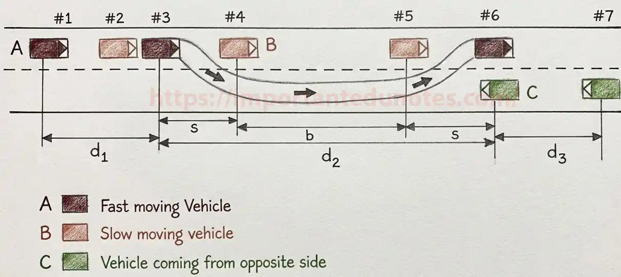
Derivation of OSD
$OSD = d_1 + d_2 + d_3$
- $d_1$ (Reaction distance): Distance traveled by the overtaking vehicle at speed $v_b$ during reaction time $t$.
$$d_1 = v_b \cdot t \quad (t \approx 2 \text{ sec})$$
- $d_2$ (Overtaking manoeuvre distance): During overtaking time $T$, the overtaking vehicle must cover the spacing $s$ behind the slow vehicle + the distance the slow vehicle travels ($v_b \cdot T$) + the spacing $s$ ahead.
$$d_2 = v_b \cdot T + 2s$$Using kinematics (since overtaking vehicle accelerates at $a$):$$d_2 = v_b \cdot T + \frac{1}{2}aT^2 \implies T = \sqrt{\frac{4s}{a}}$$Minimum spacing: $s = 0.2v_b + 6$ metres (where $v_b$ in kmph).
- $d_3$ (Oncoming vehicle distance):
$$d_3 = v \cdot T$$
OSD (one-way road) = d₁ + d₂ [d₃ = 0]
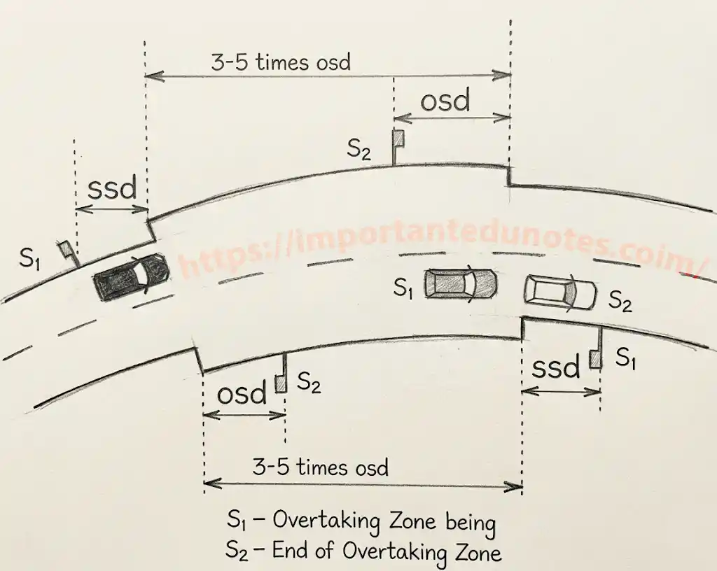
Minimum Length of Overtaking Zone
- Minimum length = $3 \times OSD$
- Desirable length = $5 \times OSD$
1. PIEV Theory
The total reaction time of a driver is the time from the instant the object is visible to the instant the brakes are applied. The PIEV theory breaks this into four sequential stages:
| Stage | Full Name | Description |
|---|---|---|
| P | Perception | Time required by the eyes to transmit the image to the brain. |
| I | Intellection | Time required by the brain to understand/interpret the situation (recognizing the hazard). |
| E | Emotion | Time elapsed during psychological sensations like fear, anger, or panic affecting decision-making. |
| V | Volition | Time required for the brain to command muscles and physically apply the brakes. |
Example: A driver at 80 km/h sees a fallen tree — Perception (sees the object) → Intellection (realizes it blocks the road) → Emotion (feels fear of crashing) → Volition (moves foot from accelerator to brake pedal). Total PIEV time is typically taken as 2.5 seconds for design purposes.
2. Types of Sight Distances
- Stopping Sight Distance (SSD): Minimum sight distance to stop safely without hitting a stationary object.
- Overtaking Sight Distance (OSD): Distance required to safely overtake a slower vehicle against oncoming traffic.
- Intermediate Sight Distance (ISD): Defined as $2 \times SSD$; used when OSD cannot be provided.
- Intersection Sight Distance: Required for vehicles to safely enter or cross an intersection.
3. Stopping Sight Distance (SSD)
Definition: SSD is the minimum length of road visible ahead to a driver to safely bring a vehicle traveling at design speed to a complete stop before hitting a stationary object.
Factors Affecting SSD:
- Total reaction time of driver (PIEV time, usually 2.5 s).
- Design speed of the vehicle ($v$).
- Efficiency of brakes.
- Frictional resistance between road and tires ($f$).
- Gradient of the road.
4. Derivation of SSD at a Level Road
SSD consists of two components:
- Lag Distance: Distance traveled at uniform design speed $v$ during total reaction time $t$.
$$\text{Lag Distance} = v \cdot t$$
- Braking Distance: By equating kinetic energy to work done against friction:
$$\frac{1}{2}mv^2 = f \cdot m \cdot g \cdot d \implies d = \frac{v^2}{2gf}$$
Where $v$ is in m/s, $t$ is in seconds (2.5 s), $g = 9.81$ m/s², $f$ is the coefficient of longitudinal friction (typically 0.35 to 0.40).
Chapter 2: Highway Engineering
Advantages of Road Transport
- Door-to-Door Service: Unlike railways or airways, road transport provides maximum flexibility offering point-to-point and door-to-door service without needing transit changes.
- Flexibility: Routes, timings, and speeds can be adjusted easily according to individual needs.
- Feeder System: Roadways act as a vital feeder system for other modes of transport (airports, railway stations, and harbors).
- Cost-Effective for Short Distances: For short-haul trips, road transport is faster and more economical compared to rail or air.
- Lower Initial Investment: The capital cost for constructing roads and acquiring vehicles is significantly lower than that of railways or airways.
Relevancy of Road Transportation in Nepal
- Topographical Constraints: Over 80% of Nepal consists of rugged hills and high mountains. Constructing railways or developing navigable waterways is technically extremely difficult and economically unviable in such terrain.
- High Cost of Air Travel: Air transport is prohibitively expensive for the general public and heavily dependent on clear weather conditions.
- Socio-Economic Integration: Roads connect remote, isolated villages with district headquarters and urban centres, providing access to hospitals, schools, and markets.
- Agricultural and Tourism Development: Nepal’s economy heavily relies on agriculture and tourism. Roads enable farmers to transport perishable goods quickly and allow tourists to access remote scenic destinations.
- Strategic and Administrative Control: A well-connected road network is crucial for administrative efficiency, national security, and rapid disaster response during earthquakes or landslides.
John Macadam (1756–1836) is considered the pioneer of modern road construction because he revolutionized road building by introducing a scientific approach that is the foundation of modern flexible pavements today.
Why he is a pioneer:
- He proved that the natural subgrade soil could bear the traffic load provided it is kept well-drained and dry — eliminating the need for massive expensive stone foundations used previously.
- He introduced the concept of providing a cross-slope (camber) to the subgrade and the surface to drain rainwater efficiently.
- He used smaller, angular broken stones compacted by traffic that interlocked to form a strong, self-supporting crust.
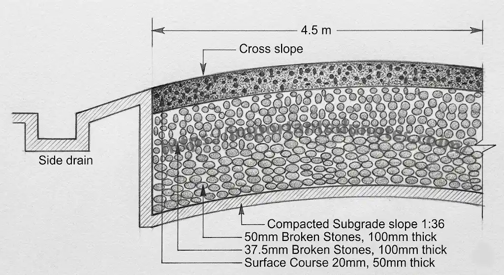
Macadam Road Construction Method
- Subgrade Preparation: The subgrade was compacted and provided with a cross slope of 1 in 36 to ensure drainage. It forms the primary load-bearing layer.
- Bottom Layer: Broken stones passing a 5 cm ring were laid to a compacted thickness of 10 cm.
- Surface Layer: Smaller broken stones passing a 3.75 cm ring were laid to a thickness of 10 cm above the bottom layer.
- Binding: No separate binding material was used initially. Angular stones interlocked under the pressure of traffic. The total thickness was kept around 25 cm, relying purely on interlocking and load dispersion through the compacted stone skeleton.
Administrative Classification (NRS 2070)
- National Highways (NH): Main arterial routes spanning the length and breadth of the country (East-West and North-South corridors). Connect national capitals, major industrial centres, and international borders.
- Feeder Roads (FR): Roads connecting district headquarters, major economic centres, and tourism hubs to the National Highways.
- District Roads (DR): Important intra-district roads connecting villages and towns to the district headquarters or nearest feeder roads.
- Urban Roads (UR): Roads serving urban municipalities and city areas.
Technical Classification (based on traffic volume in PCU/day)
| Class | Traffic Volume (PCU/day) | Type |
|---|---|---|
| Class I | > 20,000 | Divided Carriageway / Expressways |
| Class II | 5,000 – 20,000 | Two-lane roads |
| Class III | 2,000 – 5,000 | Intermediate / Single lane |
| Class IV | < 2,000 | Single lane / Earthen track |
Relevance in the Present Context
- Fund Allocation: Provides a clear framework for budget distribution. National and Feeder roads are maintained by the central government (DoR), while District and Urban roads are managed by local/provincial governments (DoLI).
- Design Standardization: Classification dictates geometric design standards (Right of Way, design speed, width) ensuring uniform safety and capacity across similar road types.
- Strategic Planning: Helps policymakers prioritize road network expansion and upgrading based on administrative hierarchy and traffic demand.
The Nepal Urban Road Standard (NURS) classifies urban roads based on their function within the city:
- Expressways / Arterial Roads: High-capacity urban roads designed to carry large volumes of traffic over long distances within or across a city. They prioritize mobility over access to adjoining properties.
- Sub-Arterial Roads: Connect arterial roads to areas of major traffic generation. Offer a slightly lower level of mobility but handle significant cross-city traffic.
- Collector Roads: Collect traffic from local residential roads and distribute it to sub-arterial and arterial roads. Provide a balance between mobility and direct access to properties.
- Local Roads: Primarily provide direct access to abutting properties. Speed limits are low, and through-traffic is discouraged.
- Paths / Alleys (Goreto / Galli): Narrow lanes primarily meant for non-motorized traffic, pedestrians, and two-wheelers in densely populated older city cores.
Highway Alignment: The position or layout of the centre line of the highway on the ground is called Highway Alignment. It includes the horizontal alignment (straight paths and curves in a horizontal plane) and vertical alignment (gradients and vertical curves).
Requirements of an Ideal Highway Alignment — “S-E-S-E”
- Short: The alignment between two terminals should be as straight and short as possible. A shorter route saves construction cost, vehicle operating time, and fuel. Unnecessary detours must be avoided.
- Easy: The alignment must be easy to construct and maintain. It should be easy for the operation of vehicles — gradients should be gentle, and curves should have adequate radii to prevent the need for frequent gear shifts or severe braking.
- Safe: The alignment must be safe for driving. It should provide adequate sight distances (SSD, OSD), stability against landslides in hills, and safe cross-sections. Sharp curves on steep gradients must be avoided.
- Economical: The total cost — which includes initial construction cost, maintenance cost, and vehicle operating cost — should be minimized. The alignment should balance earthwork (cutting and filling) to reduce expenses.
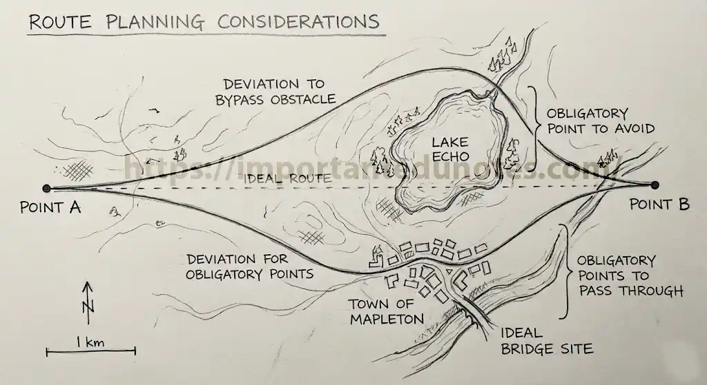
Factors Controlling Highway Alignment Selection
- Obligatory Points:
- Points the road MUST pass through: Bridge sites (narrow river cross-sections with firm banks), intermediate towns, mountain passes (saddles).
- Points the road MUST AVOID: Costly agricultural land, religious/historical monuments, unstable geological zones, marshes, and lakes.
- Traffic: The alignment should suit the desired line of traffic origin and destination, touching major traffic generation nodes without unnecessary detours.
- Geometric Design Constraints: Design speed, maximum gradient, minimum radius of curve, and required sight distance strictly govern the alignment. To maintain a gentle gradient in hills, the alignment must artificially increase its length (development of route using hairpin bends).
- Economical Factors: The alignment should ensure a balance in earthwork (volume of cut ≈ volume of fill). It should be close to construction materials and water sources.
- Other Considerations: Drainage (avoiding flood-prone areas), political factors, and environmental impacts (protecting forests and wildlife).
Highway route location is the systematic process of determining the final alignment of a road on the ground. Engineering surveys are conducted in four consecutive, structured stages:
- Map Study (Office Study):
- Process: Topographic maps are studied in the office to identify major obligatory points, river crossings, mountain passes, and contour patterns.
- Output: Several tentative alternative routes are sketched on the map without going to the field.
- Reconnaissance Survey (Field Inspection):
- Process: An initial field inspection of the tentative routes using simple instruments (Abney level, compass, altimeter).
- Utilization from Map Study: The map study’s tentative routes are verified on the ground. Actual soil conditions, approximate gradients, rock outcrops, and unmapped obstacles are collected.
- Output: Unfeasible routes are eliminated. The best one or two routes are selected for further detailed study.
- Preliminary Survey (Instrumental Survey):
- Process: A rigorous instrumental survey (Theodolite, Total Station, Leveling instruments) along the selected best routes from the reconnaissance phase.
- Utilization from Reconnaissance: The rough route is accurately mapped. Detailed longitudinal profiles, cross-sections, and soil testing are conducted.
- Output: A comparative analysis (cost, earthwork) is done to finalize the single best optimal alignment on paper.
- Detailed Survey / Location Survey (Staking on Ground):
- Process: The finalized paper alignment is transferred and pegged directly onto the ground with detailed leveling and cross-sectioning at 10–20 m intervals.
- Utilization from Preliminary: The paper alignment is translated into physical reality using pegs, benchmarks, and reference pillars.
- Output: Detailed Project Report (DPR), final working drawings, and exact Bill of Quantities (BOQ) ready for construction bidding.
Definition: A hill road is defined as a road passing through mountainous or hilly terrain where the transverse slope (cross slope) of the land is generally greater than 25%.
Special Considerations and Construction Challenges
- Stability: The primary challenge is maintaining the stability of hill slopes. Excavation alters the natural equilibrium, leading to landslides and rockfalls. Retaining walls and breast walls are heavily required.
- Drainage: Hills experience heavy runoff. Complex drainage structures (catch-water drains, cross drains/culverts, scuppers) must be designed to prevent washing away of the road formation.
- Geometric Design Restrictions: Achieving ideal gradients and sight distances is very difficult. Sharp curves, hairpin bends, and steep gradients are unavoidable. Extra widening at curves is mandatory.
- Construction Logistics: Accessing the site, mobilizing heavy equipment, managing excavated earth (spoil disposal) without damaging the valley below are massive challenges.
Factors Controlling Alignment of Hill Roads
- Topography (Saddles and Passes): The road must target natural depressions (saddles or passes) in the ridges to cross mountain ranges with minimum earthwork.
- Geological Conditions: Alignment should be located where the dip of the rock strata is inclined inwards (into the hill) rather than outwards (towards the valley) to prevent slipping. Fault zones must be avoided.
- Climatic Conditions: Slopes facing the sun (southern slopes in Nepal) are preferred as they dry faster after rain and melt snow quicker — maintaining year-round operability.
- River Crossings: Alignments should cross rivers at right angles and at locations where the banks are rocky and stable, minimizing bridge length and cost.
- Temperature: In high-altitude areas, low temperatures lead to snowfall and frost action. Alignments are preferred on sun-facing slopes (South-facing in Nepal) to ensure quick snow melting. Routes are generally kept below the permanent snow line to keep the road operational year-round.
- Rainfall: Areas with excessive rainfall are prone to severe erosion and landslides. The alignment must avoid highly saturated zones, deep valleys prone to flash floods, and must incorporate extensive drainage systems.
- Atmospheric Pressure: At high altitudes, atmospheric pressure and oxygen levels drop. This drastically reduces combustion efficiency and pulling power of vehicular engines. Consequently, the maximum allowable gradients must be kept flatter than those in plains to prevent vehicle stalling on upgrades.
- Geological Conditions: Road alignment is highly influenced by rock types and strata orientation. Alignments must avoid active fault lines, shear zones, and areas with a history of landslides. It is structurally safer to align the road where the dip of geological strata is inclined towards the hill rather than towards the valley.
1. River Route (Valley Route)
The alignment is laid out parallel to the course of a river or stream flowing in the valley.
- Basic Consideration: Must be kept safely above the High Flood Level (HFL) of the river.
- Merits: Provides a very gentle and easy gradient following the river’s natural slope; effectively connects major populations as most hill settlements are near water sources in valleys.
- Demerits: Requires numerous cross-drainage structures and major bridges; high risk of damage during floods and riverbank scouring.
2. Ridge Route (Watershed Route)
The alignment is laid out along the crest or ridge of a mountain range, tracing the watershed line.
- Basic Consideration: Reaching the ridge from the valley requires a steep initial gradient or development of route length using hairpin bends.
- Merits: Minimal cross-drainage structures needed (water flows away on both sides); completely safe from river floods; usually provides stable ground.
- Demerits: Initial climb involves very steep gradients and expensive earthwork; severe scarcity of water during construction; often misses major settlements in valleys below.
| Feature | River Route | Ridge Route |
|---|---|---|
| Location | Follows valley bottom along a river | Follows the crest of the mountain/hill |
| Gradient | Gentle and easy | Steep during initial climb, then gentle |
| Cross-Drainage | Maximum (requires many bridges) | Minimum (no streams cross the crest) |
| Flood Risk | High risk | Zero risk |
| Settlements | Connects most valley settlements | Often remote from major populations |
Chapter 3: Geometric Design of Highway
Geometric design of a highway refers to the physical proportioning of visible elements such as cross-sections, horizontal and vertical alignments. The primary objective is to provide optimum efficiency in traffic operations with maximum safety at a reasonable cost.
Factors Controlling Geometric Design
- Design Speed — most important factor governing almost all other design elements.
- Topography (Terrain) — dictates alignment and gradients.
- Traffic Factors — volume, composition, and capacity requirements.
- Design Vehicle — dimensions, weight, and operating characteristics.
- Environmental Factors — aesthetics, noise pollution, landscaping.
- Economics — capital cost and maintenance cost.
How Each Factor Affects Design
Design Speed: Directly dictates sight distances (SSD, OSD), radius of horizontal curves, superelevation, transition curve length, and length of vertical curves. Higher design speed requires wider lanes, gentler curves, and flatter gradients, increasing safety but also increasing construction cost.
Design Vehicle: The physical dimensions of the heaviest/largest vehicle expected govern the design. Width affects lane and shoulder width; Length affects turning radius and extra widening; Height dictates vertical clearance under bridges; Weight affects pavement thickness and maximum gradient.
Topography (Terrain): Terrain is classified as Plain (0–10% cross slope), Rolling (10–25%), Mountainous (25–60%), and Steep (>60%). Mountainous and steep terrains require sharp curves, steep gradients, hairpin bends, and heavy earthwork, which significantly restricts design speed compared to plain terrain.
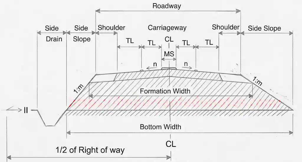
Cross-sectional Elements of a Typical Highway
- Carriageway (Pavement): The paved portion intended for vehicular traffic. Width depends on number of lanes and design vehicle width.
- Shoulders: Provided along the edge of the carriageway for emergency parking, lateral support of pavement, and safety.
- Camber (Cross slope): The transverse slope provided to drain off rainwater from the road surface (highest at crown, sloping down to edges).
- Medians (Traffic Separators): Provided in divided highways to separate opposing traffic streams, preventing head-on collisions.
- Side Slopes (Cut/Fill Slopes): Provided to ensure the stability of earthwork (e.g., 1:2 for filling, 1:1 for cutting in soil).
- Right of Way (ROW): Total land area acquired for construction and future expansion of the road.
- Drainage/Ditches: Provided at the edges to carry away surface runoff.
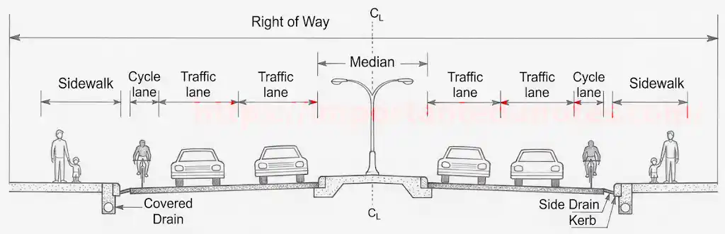
Additional Elements in Urban Roads
- Sidewalks (Footpaths): Elevated areas for pedestrian safety, separated from the carriageway by kerbs.
- Kerbs: Vertical or sloping boundaries separating the carriageway from sidewalks.
- Cycle Tracks: Dedicated lanes for bicycles.
- Parking Lanes: Space provided for parallel or angle parking adjacent to the carriageway.
- Bus Bays: Recessed areas for buses to stop without disrupting traffic flow.
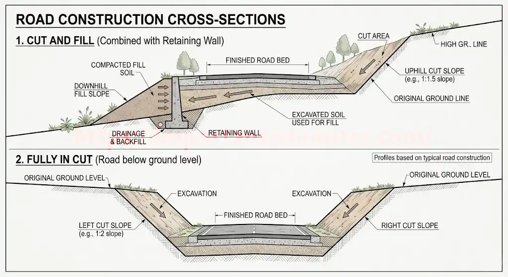
- Cut and Fill Section (Partial Cutting and Filling): The road is benched into the hillside. Half the road width is formed by excavating the hill (cut) and the excavated material is used to construct the other half on the valley side (fill). This is the most common and economical cross-section as it balances earthwork. Retaining walls are often provided on the valley side and breast walls on the hill side.
- Fully in Cutting (Trench Type): The entire cross-section is carved into the hillside. Used where the valley side is too steep or unstable to support a fill section, or when the road passes through a ridge. Requires heavy excavation and good side drainage.
- Fully in Filling (Embankment): The entire road is built upon compacted fill material. Rarely used in hill roads, but applicable when the road passes through a valley, river crossing, or low-lying depression between hills.
- Half Tunnelling / Rock Ledge: The road is carved out of a sheer vertical rock face, creating an overhang (canopy) of natural rock above the road. Used in extremely steep, rocky terrains where cutting the entire vertical face is impractical, expensive, or would cause massive instability.
Definition: Camber (or cross slope) is the transverse slope provided to the road surface to drain off rainwater from the carriageway. It is usually highest at the centre (crown) and slopes down towards the edges.
Types of Camber
- Parabolic/Elliptical Camber: The profile is curved (parabola). Favorable for fast-moving vehicles as it provides a smooth transition from centre to edge, but difficult to construct accurately.
- Straight Line Camber: Consists of two straight slopes joining at the crown. Easy to construct; best suited for cement concrete pavements.
- Composite Camber: Central part is parabolic and edges are straight lines — combining the advantages of both types.
How Camber Value is Decided
- Type of Pavement Surface: Smoother, impervious surfaces (concrete or bitumen) require less camber (1.5–2%) because water flows easily. Rough surfaces (WBM or gravel) require more camber (2.5–4%) to prevent water soaking in.
- Amount of Rainfall: Areas with heavy rainfall require steeper camber for quick drainage.
Advantages of Providing Camber
- Quickly drains surface water, preventing slipping and skidding of vehicles.
- Prevents water from percolating into the subgrade, protecting the pavement structure from weakening and stripping.
- Improves the aesthetic appearance of the road.
Disadvantages of Heavy/Steep Camber
- Vehicles tend to slip or drag towards the edges, especially on wet surfaces.
- Uneven wear and tear of tires.
- Drivers tend to drive strictly along the centre line to avoid lateral tilt, reducing the effective usable width of the pavement.
- Causes discomfort to passengers and requires more steering effort.
Difference Between Camber and Superelevation
| Feature | Camber | Superelevation |
|---|---|---|
| Location | Provided on straight stretches of road | Provided on horizontal curves |
| Direction of slope | Slopes downwards from the centre (crown) to both edges | Entire width slopes upwards from inner edge to outer edge |
| Purpose | To drain rainwater off the road surface | To counteract centrifugal force and prevent overturning/skidding |
Superelevation ($e$): The inward transverse inclination provided to the cross-section of a carriageway at horizontal curves. The outer edge is raised with respect to the inner edge to counteract the centrifugal force acting on vehicles.
Equilibrium Superelevation: The condition where the centrifugal force is fully counteracted by the component of the vehicle’s weight alone, meaning the lateral friction developed between tires and road is zero ($f = 0$). Pressure on all tires is equal.
Derivation of Superelevation Expression
Let a vehicle of weight $W$ move with velocity $v$ (m/s) on a curve of radius $R$. Centrifugal force: $P = Wv^2/gR$. Superelevation angle: $\theta$, so $e = \tan\theta$. Lateral friction: $f$.
Resolving forces parallel to the inclined road surface for equilibrium:
Dividing by $W\cos\theta$, and noting $P/W = v^2/gR$, $\tan\theta = e$, and neglecting the very small term $(P/W)\tan\theta$:
Substituting $v = V/3.6$ (where $V$ is in km/hr) and $g = 9.81$ m/s²:
Design Steps of Superelevation (NRS Method)
- Calculate superelevation for 75% of design speed neglecting friction ($f = 0$): $e_{calc} = V^2/(225R)$.
- If $e_{calc} \le e_{max}$, provide $e_{calc}$. (where $e_{max} = 0.07$ for plain/rolling terrain, $0.10$ for hilly terrain).
- If $e_{calc} > e_{max}$, provide maximum superelevation $e = e_{max}$ and check friction: $f_{calc} = V^2/(127R) – e_{max}$.
- If $f_{calc} \le 0.15$ (safe limit), the design is acceptable.
- If $f_{calc} > 0.15$, restrict the allowable speed: $V_a = \sqrt{127R(e_{max} + 0.15)}$.
Methods of Attaining Superelevation
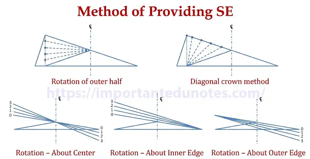
- Elimination of crown of the cambered section: First, the outer half of the camber is rotated upwards until it matches the inner slope, making a straight line slope across the full width.
- Rotation of the pavement cross-section:
- About the Centre Line: Depressing the inner edge and raising the outer edge by $E/2$. Earthwork is balanced; widely used.
- About the Inner Edge: Raising the centre line by $E/2$ and outer edge by $E$. Used in flat terrains to avoid drainage problems.
- About the Outer Edge: Depressing the inner edge. Used in congested urban areas where the road level is fixed by kerbs.
Reasons/Necessity for Extra Widening
- Mechanical Off-tracking: Because of the rigidity of the wheelbase, the rear wheels of a vehicle do not follow the same path as the front wheels on a curve — they track inside. The pavement must be wider to accommodate this off-tracking.
- Psychological Factors: Drivers naturally maintain greater clearance from edges and opposing vehicles while negotiating a curve, effectively reducing the usable width of a straight-designed road.
- Visibility: To ensure higher visibility and adequate sight distance across the curve for both approaching vehicles.
- Steering Difficulties: Difficulty in steering long wheelbase vehicles tightly along curves requires additional physical width.
Advantages of Providing a Shoulder
- Provides space for emergency parking of disabled vehicles without blocking traffic.
- Provides lateral structural support to the pavement edges, preventing edge cracking.
- Enhances safety by providing a recovery space for errant vehicles.
- Provides space for traffic signs, guardrails, and utility poles.
- Increases psychological comfort and effective sight distance for drivers.
Derivation of Extra Widening ($W_e$)
$W_e = W_m + W_{ps}$
Mechanical Widening ($W_m$) Derivation: Consider a vehicle of wheelbase $l$ on a curve of radius $R$. Let $R_1$ = radius of outer front wheel, $R_2$ = radius of inner rear wheel.
Since $(R_1+R_2) \approx 2R$ and $(R_1-R_2) = W_{m1}$ per lane:
Psychological Widening ($W_{ps}$): IRC empirical formula:
Methods of Providing Extra Widening
- On Plain/Rolling Terrain: Provided equally on both the inner and outer sides ($W_e/2$ on each side).
- On Hill Roads (Sharp Curves): Provided entirely on the inner side of the curve to maintain safety and visibility — prevents the vehicle from encroaching on the precipice.
- Gradual Introduction: Extra widening is introduced gradually over the length of the transition curve, starting from zero at the tangent point to full $W_e$ at the beginning of the circular curve.
When a vehicle negotiates a horizontal curve, a Centrifugal Force ($P$) acts outwards through the centre of gravity of the vehicle:
This outward force creates two major stability issues on an un-superelevated road: tendency to overturn outwards about the outer wheels, and tendency to skid laterally outwards.
1. Condition for Overturning
Let $h$ = height of C.G. from road surface, $b$ = track width (distance between inner and outer wheels).
- Overturning moment about the outer wheel = $P \times h$
- Restoring moment due to weight = $W \times b/2$
For equilibrium: $P \cdot h = W \cdot \frac{b}{2} \implies \frac{P}{W} = \frac{b}{2h}$
If $v^2/(gR) > b/(2h)$, the vehicle will overturn outwards.
2. Condition for Lateral Skidding
Centrifugal force $P$ pushes the vehicle laterally. Maximum frictional resistance = $f \cdot W$ (where $f$ is the lateral friction coefficient, typically 0.15).
For equilibrium: $P = f \cdot W \implies P/W = f$
If $v^2/(gR) > f$, the vehicle will skid laterally outwards.
Note: Whether a vehicle overturns or skids first depends on the relationship between $b/(2h)$ and $f$. If $f < b/(2h)$, the vehicle will skid before overturning — which is the common case in passenger cars with a wide track and low C.G.
A transition curve is a curve of varying radius introduced between a straight line (tangent, $R = \infty$) and a circular curve ($R = R_c$).
Objectives of Providing a Transition Curve
- To gradually introduce the centrifugal force, preventing a sudden jerk to the passengers when entering a circular curve.
- To gradually introduce the required superelevation and extra widening over its length.
- To enable the driver to steer the vehicle comfortably into the circular curve without abruptly changing the steering angle.
- To improve the aesthetic appearance of the alignment by providing a smooth, flowing curve.
Derivation of Length of Transition Curve ($L_s$)
Criterion 1: Rate of Change of Centrifugal Acceleration
Let $C$ be the allowable rate of change of centrifugal acceleration (m/s³). The acceleration changes from 0 (on straight) to $v^2/R$ (on circular curve) over time $t = L_s/v$:
Criterion 2: Rate of Change of Superelevation
The full superelevation $E$ must be attained gradually over the length $L_s$. Let $N$ = rate of introducing superelevation (typically 1 in 150). Let total width of pavement at curve = $B = W + W_e$. If pavement is rotated about the centre line:
The larger value from all criteria is adopted as the final design length of the transition curve.
Setback Distance ($m$): The distance required from the centre line of a horizontal curve to an obstruction on the inner side to ensure adequate sight distance for safe driving.
Factors Affecting Setback Distance
- Required Sight Distance ($S$) — Stopping or Overtaking.
- Radius of the horizontal curve ($R$).
- Length of the curve ($L_c$) compared to the sight distance ($S$).
Derivation for Single-Lane Roads
Case A: $L_c > S$ (Curve length greater than sight distance)
The entire sight distance arc falls within the curve. The angle subtended: $\alpha/2 = 180 \cdot S/(2\pi R)$
Case B: $L_c < S$ (Curve length less than sight distance)
Let $\alpha’/2 = 180 \cdot L_c/(2\pi R)$. The clearance includes the middle ordinate of the curve part plus the tangential offset of the straight parts:
Derivation for Multiple-Lane Roads
The sight line is measured from the centre line of the inner lane. Let $d$ = distance from road centre line to inner lane centre line. Effective radius = $(R – d)$.
Case A ($L_c > S$):
Case B ($L_c < S$):
where $\alpha’/2 = 180 \cdot L_c / [2\pi(R-d)]$
Definition: A hair pin bend is an extreme horizontal reverse curve located on a hillside where a road reverses its direction to climb the slope. It has a minimum radius and a maximum deflection angle, physically resembling a hairpin. It is unavoidable in hill roads to gain elevation when the slope is too steep for a direct straight climb.
Elements of a Symmetrical Hair Pin Bend
A symmetrical hair pin bend consists of a central circular curve of radius $R$ and deflection angle $\Delta$, flanked by two identical transition curves of length $L_s$. Let $\alpha$ = deflection angle between the primary tangents and $\theta_s$ = spiral angle.
- Total Angle of Circular Curve ($\Delta$):
$$\Delta = (180° – \alpha) – 2\theta_s \quad \text{and} \quad L_c = \frac{\pi R \Delta}{180}$$
- Shift ($S$):
$$S = \frac{L_s^2}{24R}$$
- Total Tangent Length ($T$):
$$T = (R + S)\tan\left(\frac{180° – \alpha}{2}\right) + \frac{L_s}{2}$$
- Neck Width: The narrowest distance between the parallel roads below and above the bend:
Neck Width ≈ 2R + 2S (adjusted for side slopes)Adequate neck width is critical to prevent slope failure between the tiers.
- Total Length of Hair Pin Bend ($L_{total}$):
$$L_{total} = L_c + 2L_s$$
Gradient is the longitudinal slope provided to the formation level of a road along its alignment. It is expressed as 1 in N or as a percentage.
Types of Gradients
- Ruling Gradient (Design Gradient): The maximum gradient with which the designer attempts to design the vertical profile of the road. Ensures vehicles can climb at design speed without significant speed reduction or excessive gear shifting.
- Limiting Gradient (Maximum Gradient): A steeper gradient than the ruling gradient, permitted only for short distances where the ruling gradient is not feasible due to severe topography or high construction cost.
- Exceptional Gradient: The absolute steepest gradient allowed. Used only under unavoidable, exceptional circumstances and for very short stretches (not exceeding 100 m).
- Minimum Gradient: A flat minimum slope required strictly for longitudinal drainage of rainwater from the road surface (0.5% for concrete drains, 1.0% for soil drains).
Factors Considered in Selection of Gradient
- Nature of the Ground (Terrain): Steep terrain necessitates steeper gradients to avoid massive earthwork.
- Traffic Composition: A high percentage of heavy commercial vehicles demands flatter gradients to prevent stalling.
- Design Speed: Higher design speeds require flatter ruling gradients for safe stopping distance.
- Drainage Requirements: Minimum gradients are dictated by rainfall intensity and drain material.
- Safety and Economics: Flatter grades are safer and reduce vehicle operating costs, but may drastically increase earthwork construction costs in hilly terrain.
Definition: A momentum grade is a specific vertical alignment profile where a descending gradient (downgrade) is immediately followed by an ascending gradient (upgrade) that may be steeper than the ruling gradient.
Significance
- Utilization of Kinetic Energy: As a vehicle travels down the first slope, it gathers momentum. This acquired kinetic energy assists the vehicle in climbing the subsequent steep upgrade without the need for heavy gear shifting or immense tractive effort from the engine.
- Fuel and Time Economy: Allows vehicles to maintain a steady, continuous speed, saving fuel and reducing travel time significantly on long hilly routes.
- Economic Design: Allows the designer to adapt the road to natural “dip” topography, saving enormous costs that would otherwise be spent on massive valley filling.
- Limitation: For a momentum grade to be safe, there must be absolute, clear, unobstructed sight distance across the entire dip to prevent collisions, as vehicles move at high speeds at the valley floor.
Curve Resistance: When a vehicle negotiates a horizontal curve, its rigid wheelbase makes the wheels turn at an angle ($\alpha$) to the direction of motion. Only a portion of the tractive effort ($T\cos\alpha$) moves the vehicle forward, while a component ($T\sin\alpha$) is lost in overcoming transverse friction. This loss of tractive effort due to the turning action of wheels is called curve resistance.
Grade Compensation: The reduction in the allowable longitudinal gradient on a road section where a horizontal curve overlaps with an ascending gradient.
Causes and Reasons
- When a horizontal curve and a vertical upgrade coincide, the vehicle simultaneously experiences both grade resistance (due to gravity) and curve resistance (due to turning).
- If the gradient is already at the maximum allowable limit (Ruling Gradient), the addition of curve resistance will stall the vehicle or severely overload the engine.
- Therefore, the gradient must be flattened (compensated) at the curve so that the total resistance (grade + curve) does not exceed the resistance of the ruling gradient on a straight path.
Method of Providing Grade Compensation (NRS Formula)
- Calculate Grade Compensation (%):
Grade Compensation = (30 + R)/R — subject to maximum of 75/R (R in metres)Adopt the lesser of the two values.
- Calculate Compensated Gradient:
Compensated Grade = Original Gradient (%) − Grade Compensation (%)
- Check: Grade compensation is not required if the existing gradient is flatter than 4%. The compensated gradient should never be made less than 4%.
Vertical curves connect two intersecting gradients and are of two types: Summit Curves (convex) and Valley/Sag Curves (concave).
Significance of the Lowest Point (on Valley/Sag Curves):
- Drainage: It is the primary spot where rainwater collects. Locating it precisely is critical for designing cross-drainage structures like culverts or catch basins to prevent waterlogging of the subgrade.
- Clearance: If the valley curve passes under a bridge or overpass, the lowest point dictates the maximum vertical clearance available for traffic.
Significance of the Highest Point (on Summit Curves):
- Sight Distance: The highest point is the most critical location for checking the available Stopping Sight Distance (SSD) and Overtaking Sight Distance (OSD). The design must ensure adequate sight distance is available at this critical point.
- Clearance: If the curve passes over an underpass or tunnel, the highest point determines the structural clearance envelope required.
Chapter 4: Highway Drainage
Highway Drainage System: The complete system of structures and design provisions that collect, convey, and dispose of surface water and sub-surface moisture from the road prism, maintaining the strength and serviceability of the pavement.
Necessity and Importance
- Protect Subgrade Strength: Water is the primary enemy of roads. When the subgrade absorbs water, its bearing capacity drops dramatically, causing settlements and pavement failures (rutting, potholing).
- Prevent Pavement Distress: Standing water on the surface causes stripping of bitumen from aggregates, promotes pothole formation, and weakens the pavement structure.
- Ensure Traffic Safety: Standing water on the carriageway causes hydroplaning and reduces friction, leading to accidents.
- Prevent Slope Erosion: Uncontrolled surface water causes severe erosion of earthwork slopes (cut and fill), ultimately leading to landslides.
- Extend Pavement Life: Proper drainage is the single most effective measure to extend the design life of a road.
Components of Highway Drainage
- Surface Drainage: Side drains (roadside ditches), cross drains (culverts, causeways), catch drains, longitudinal drains.
- Sub-surface Drainage: French drains, pipe underdrains, blanket drains (filter blankets), intercepting drains.
- Cross-Drainage Structures: Bridges, culverts, causeways, and fords for stream crossings.
- Protection Structures: Retaining walls, breast walls, gabions, and slope protection works.
Differences: Surface vs. Sub-surface Drainage
| Feature | Surface Drainage | Sub-surface Drainage |
|---|---|---|
| Purpose | Removes water from the road surface and adjacent ground rapidly | Controls groundwater and seepage water below the road prism |
| Location | On the ground surface (ditches, drains) | Below the pavement or within the embankment |
| Design Basis | Based on surface runoff (rainfall intensity, catchment area) | Based on groundwater table, seepage pressure, and soil permeability |
| Key Structures | Side drains, culverts, catch drains, scuppers | French drains, pipe drains, filter blankets, intercepting drains |
| Primary Enemy | Rainwater and surface runoff | Groundwater, capillary rise, seepage |
Surface Water Collection and Disposal
In Rural Roads:
- Water from the cambered road surface drains off to both sides.
- Collected in open V-shaped or trapezoidal side drains (roadside ditches) running parallel to the road.
- Side drains carry water to natural streams or valleys through cross-drainage structures (culverts).
- In hilly areas, catch drains are provided uphill of the cut slope to intercept hill runoff before it reaches the road.
In Urban Roads:
- Water drains off the cambered carriageway towards the kerbs on both sides.
- Water flows along the kerb-gutter channel to street inlets spaced at regular intervals.
- Street inlets collect the water and direct it into underground storm sewers.
- Underground pipes convey the water to natural streams, retention ponds, or central drainage outfalls.
Design Procedure for a Surface Drainage System
- Determine the Catchment Area: Define the total area contributing runoff to the drainage section being designed.
- Estimate Design Discharge: Calculate the peak storm water runoff using the Rational Method: $Q = CiA/360$ (m³/s).
- Select Drain Type and Shape: Choose appropriate drain shape (V-shape, trapezoidal, rectangular) based on land availability, terrain, and maintenance requirements.
- Design Drain Dimensions: Using Manning’s equation ($Q = AR^{2/3}S^{1/2}/n$), calculate the required channel area for the design discharge. Ensure flow velocity is between the non-silting and non-scouring limits.
- Provide Adequate Gradient: Drain must have a minimum gradient (0.5% for concrete, 1% for soil) to ensure self-cleaning velocity.
- Design Outlet Structures: Provide properly sized and protected outlets to prevent erosion at the discharge point into natural streams.
Causes of Moisture Variation in Subgrade Soil
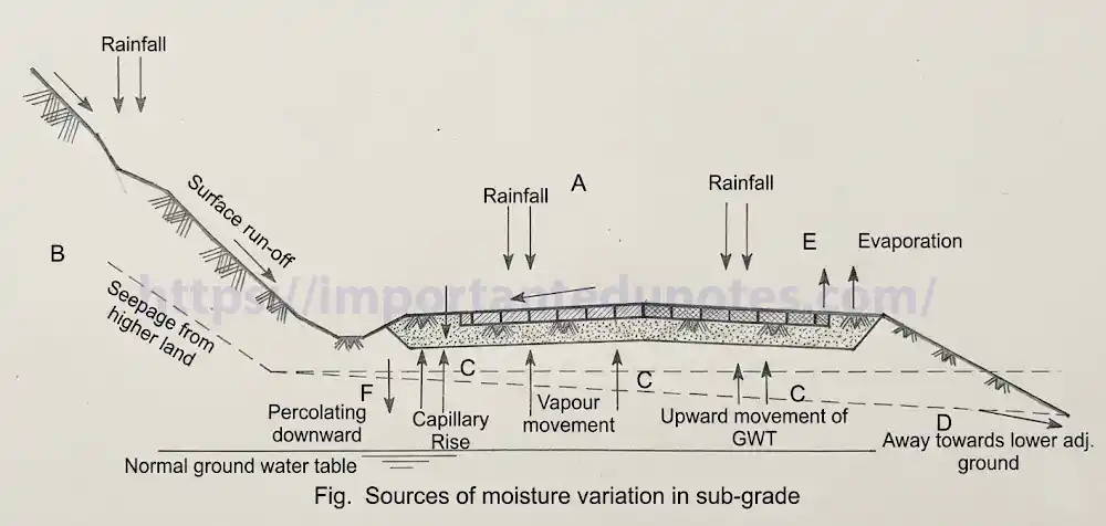
- Rainfall and Surface Infiltration: Direct precipitation percolates through cracks in the pavement or along the pavement edges into the subgrade.
- Capillary Rise: In fine-grained soils (silts, clays), water rises from the groundwater table through capillary action, increasing moisture well above the water table level.
- Seepage: Groundwater from adjacent hillsides or high-lying areas seeps laterally and vertically into the road prism.
- Variations in Groundwater Table: Seasonal fluctuations in the groundwater table directly affect subgrade moisture content.
- Condensation: Temperature differences between the warm subgrade and cool pavement cause water vapor to condense inside the pavement structure.
Control of Moisture Variation
- Surface Drainage: Effective side drains prevent surface water from percolating into the subgrade.
- Sub-surface Drainage: French drains and pipe underdrains lower the groundwater table and intercept seepage.
- Capillary Cut-off: Providing a layer of coarse granular material (gravel) above the water table level as a capillary break blanket interrupts capillary rise.
- Waterproof Blankets: Bituminous or geosynthetic membranes placed between pavement layers prevent surface water penetration.
- Stabilization: Treating the subgrade soil with lime or cement to reduce its water sensitivity.
Steps for Design of Side Drains
- Delineate the catchment area contributing runoff to each section of the side drain.
- Estimate the design peak discharge using the Rational Method: $Q = CiA/360$ m³/s.
- Determine the available longitudinal slope of the drain (typically 0.5% minimum to 5% maximum).
- Choose the drain cross-section shape (V-shape for low flow, trapezoidal for higher flows).
- Apply Manning’s equation to size the drain so that the design discharge is carried without overflowing and at a self-cleaning velocity (0.6–3.0 m/s).
- Select the drain lining material (concrete, stone masonry, or open earth) based on flow velocity and maintenance considerations.
- Design the outlet protection (scour protection/riprap) at the discharge point.
Sub-surface Drainage System: The system of sub-surface drains, filters, and associated structures designed to intercept groundwater and seepage water before it reaches and weakens the subgrade, or to lower a high water table below the critical zone of the pavement structure.
Importance
- Prevents softening and loss of bearing capacity of the subgrade soil due to saturation.
- Controls capillary rise from the water table, which can cause frost heaving in cold climates and subgrade weakening in all climates.
- Prevents hydrostatic pressure buildup within the embankment, which can cause slope failures.
- Significantly extends the life of the pavement by maintaining the subgrade in a stable, well-drained condition.
Methods to Control Seepage and Lower Water Table
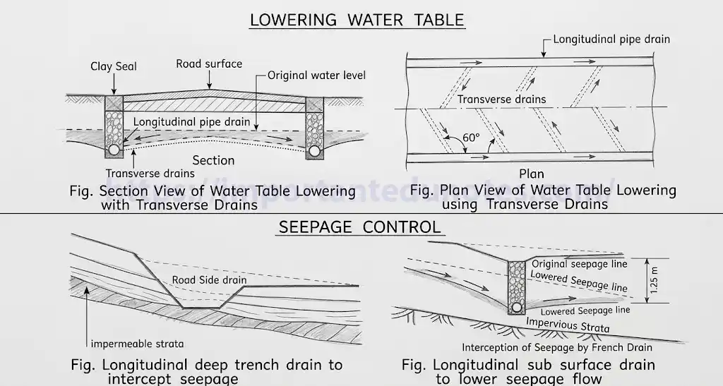
- Intercepting Drain (Cut-off Drain): A trench filled with permeable granular material (gravel/rubble) with a perforated pipe at the bottom. Placed on the uphill side of the road cutting to intercept seepage water flowing from the hillside before it reaches the road formation.
- French Drain (Rubble Drain): A trench excavated below the pavement structure, filled with coarse gravel/rubble, sometimes with a perforated pipe at the bottom. Water enters through the voids between gravel particles and is conveyed away. Used to lower a high water table below the pavement level.
- Pipe Underdrain (Longitudinal Drain): A perforated or slotted pipe laid in a gravel-filled trench alongside or below the pavement. The perforations allow groundwater to enter and the pipe conveys it to an outlet. More efficient than simple rubble drains.
- Blanket Drain (Filter Blanket): A layer of well-graded granular material (free-draining crushed stone) placed horizontally below the pavement structure. Acts as both a drainage layer and a filter — preventing migration of fine subgrade particles into the gravel while conveying water to the edge drains.
Cross-Drainage Structure: A hydraulic structure constructed across a road to allow the natural flow of water (stream, nala, or drainage channel) to pass under, through, or over the road without interruption, while the road traffic continues to flow safely.
Types and Applications
- Culvert: A small, enclosed cross-drainage structure with a span less than 6 m. Used for minor streams and nalas crossing the road. Types include box culverts (rectangular RCC box), pipe culverts (circular RCC/HDPE pipes), arch culverts (stone or brick arch), and slab culverts. Used where the water discharge is low and the road embankment height is sufficient.
- Bridge: A cross-drainage structure with a span exceeding 6 m, designed to carry the road over a larger stream, river, valley, or another road. Classified into small bridges (6–30 m), major bridges (>30 m), and long bridges (>120 m).
- Causeway (Submersible Bridge/Irish Bridge): A low-lying structure where the road crosses a stream at the stream bed level or slightly above. During floods, water flows over the top of the causeway. The road surface is hardened and scour-resistant. Used in low-traffic rural roads crossing seasonal streams where the road can temporarily close during high floods.
- Vented Causeway: A causeway with vents (openings/pipes) below the road surface to allow low normal flows to pass without overtopping. During major floods, water overtops the road surface. Better than a plain causeway as normal traffic is unaffected during smaller events.
- Ford: The simplest cross-drainage — the road simply dips down to the stream bed level and vehicles cross through the shallow flowing water directly. No structure is provided. Used only in very low-traffic minor rural roads crossing very shallow, stable streams.
- Catch Drains (Hill Drains): In hill roads, the excavated cut slope above the road can collect large volumes of rainwater running down the hillside. If not intercepted, this water erodes the cut slope, saturates the subgrade, and can destabilize the entire road formation. Catch drains are provided at the top and on the benches of the cut slope to intercept runoff from the hill above the road and divert it safely to natural drainage channels before it reaches the road surface.
- Causeways: In hilly terrain, numerous small seasonal streams and nalas cross the road alignment. Building full bridges or culverts for every minor seasonal crossing is extremely expensive and sometimes unnecessary. Causeways are economical alternatives that allow seasonal streams to flow over the road during floods while permitting normal traffic use for the majority of the year.
- Energy Dissipating Structures: On steep hill roads, water collected by side drains or chutes must be discharged rapidly over steep slopes. When water exits a steep drain at high velocity, it causes severe scouring, erosion, and undermining of the slopes and drain outlets. Energy dissipating structures (drop structures, aprons, check dams, and stilling basins) reduce the flow velocity and dissipate the kinetic energy of the water before it reaches erodible soil, preventing scour damage.
- Retaining Walls: In hill road construction, heavy cutting on the upper side and filling on the lower side creates steep, often unstable slopes. Retaining walls are gravity or reinforced concrete structures that support the fill embankment on the valley side and the cut face on the hill side, preventing the movement of earth and maintaining the stability of the road prism.
- Gully Control Structures: In hilly areas, concentrated surface runoff causes deep channels (gullies) to form on slopes. If a gully develops near a road, it can progressively erode the slope and eventually undermine the road formation. Gully control structures (check dams of stone masonry, log dams, gabion weirs) are placed across the gully channel to slow water velocity, cause deposition of sediment, and stop the regressive head-cutting of the gully.
Chapter 5: Highway Materials
Highway Material: Materials which possess quality levels sufficient for their use in various pavement structures. They are primarily categorized into: (i) Mineral Materials (sub-grade soil, aggregates), (ii) Binding Materials (bitumen, tar, cement, lime), and (iii) Other Materials (additives, fillers, geosynthetics).
Materials in Different Pavement Layers
- Sub-grade (Bottom Layer): The foundational layer consisting of natural or compacted local soil. The material should have high stability, good drainage, and minimal volume change under moisture variations. Its strength is characterized by the CBR value.
- Sub-base Course: Constructed using lower-quality, cheaper materials like granular aggregates, gravel, crushed stone, or locally available stabilized soil (lime or cement-stabilized). It prevents intrusion of sub-grade soil into the base course and improves drainage.
- Base Course: The primary load-distributing layer. Constructed using hard, durable materials like crushed stone aggregates, Water Bound Macadam (WBM), or Wet Mix Macadam (WMM). Lean concrete (DLC) is used in rigid pavements.
- Surface/Wearing Course (Top Layer): The topmost layer in direct contact with traffic. Must be tough, abrasion-resistant, and water-tight.
- Flexible pavements: Bituminous mixes (Asphalt Concrete, Dense Bituminous Macadam).
- Rigid pavements: Pavement Quality Concrete (PQC).
Sub-grade soil is the supporting structure on which the pavement rests. The desirable properties include:
- Adequate Stability: Sufficient resistance to permanent deformation under the load transmitted through the pavement layers. Measured by CBR or unconfined compressive strength.
- Incompressibility: Should not undergo substantial settlement or consolidation when subjected to vehicular traffic.
- Permanence of Strength: The soil must retain its strength and load-bearing capacity over time regardless of seasonal moisture variations.
- Minimum Volume Change: Should not exhibit excessive swelling or shrinkage during wet and dry weather cycles (low expansion/shrinkage potential). Expansive clays are undesirable.
- Good Drainage: Should allow for the easy drainage of water to prevent saturation, which drastically reduces soil strength and bearing capacity.
- Ease of Compaction: The soil should be easily compactable at optimum moisture content (OMC) to achieve high density, providing good structural support.
Preparation of Specimen
- The soil is sieved through a 20 mm IS sieve.
- The soil is mixed with water corresponding to its Optimum Moisture Content (OMC) as determined by Proctor’s test.
- The specimen is compacted in a standard cylindrical CBR mould (inner diameter 150 mm, height 175 mm) fitted with a spacer disc to achieve a 127.3 mm specimen height.
- It is dynamically compacted in layers (light compaction: 3 layers, 56 blows per layer; heavy compaction: 5 layers, 56 blows per layer) using a standard rammer.
- If soaking is required to simulate the worst moisture condition, the specimen is submerged in water for 4 days with surcharge weights placed on top.
Method of Conducting the CBR Test
- The mould with the compacted specimen is placed on the lower plate of the testing machine.
- Annular surcharge weights (usually 2.5 kg each, minimum 5 kg total) are placed on the surface to simulate the weight of overlying pavement layers.
- A cylindrical penetration plunger (50 mm diameter) is brought into contact with the soil surface, and the dial gauge is set to zero.
- Load is applied so that the plunger penetrates the soil at a uniform rate of 1.25 mm/minute.
- Load readings are recorded at standard penetrations of 0.5, 1.0, 1.5, 2.0, 2.5, 3.0, 4.0, 5.0, 7.5, 10.0, and 12.5 mm.
- A load vs. penetration curve is plotted. If the initial curve is concave upwards, a zero correction is applied.
- The CBR value is calculated for 2.5 mm and 5.0 mm penetration:
CBR (%) = (Measured Load / Standard Load) × 100Standard loads: 1370 kg for 2.5 mm; 2055 kg for 5.0 mm penetration. The higher of the two values governs.
Desirable Properties of Road Aggregates
- Strength: Resistance to crushing under gradually applied loads from heavy traffic.
- Hardness: Resistance to abrasive action (wear and tear) caused by vehicle tires.
- Toughness: Resistance to sudden impact or shocks caused by heavily loaded vehicles moving at high speeds.
- Durability (Soundness): Resistance to disintegration due to weathering actions (freezing-thawing, wetting-drying).
- Shape Factor: Aggregates should ideally be cubical/angular. Excessive flaky or elongated particles break easily and produce weaker mixes.
- Adhesion (Stripping Resistance): High affinity to bitumen to prevent stripping of the bituminous film in the presence of water.
Laboratory Tests on Road Aggregates
| Property Tested | Test Name | Key Parameter Measured |
|---|---|---|
| Strength | Aggregate Crushing Test | Aggregate Crushing Value (ACV) % |
| Hardness | Los Angeles Abrasion Test | Los Angeles Abrasion Value (LAAV) % |
| Toughness | Aggregate Impact Test | Aggregate Impact Value (AIV) % |
| Durability | Soundness Test (Na₂SO₄/MgSO₄) | Loss in weight % |
| Shape | Flakiness Index and Elongation Index Test | FI % and EI % |
| Water Absorption | Specific Gravity & Water Absorption Test | % water absorption |
| Adhesion | Stripping / Adhesion Test | % coating retained after water immersion |
Significance: The Aggregate Impact Test determines the toughness of aggregates — their resistance to fracture under sudden impacts or shocks from vehicular movement. Lower AIV = tougher aggregate.
Procedure
- The aggregate sample passing through a 12.5 mm IS sieve and retained on a 10 mm IS sieve is washed, oven-dried, and used for the test.
- The sample is filled into a cylindrical measure in three equal layers, each tamped 25 times with a standard tamping rod. The weight of this sample is recorded ($W_1$).
- The aggregate is transferred to the cup of the aggregate impact testing machine.
- A standard metal hammer (13.5 to 14.0 kg) is allowed to fall freely from a height of 380 ± 5 mm onto the aggregates.
- The sample is subjected to exactly 15 blows.
- The crushed aggregate is removed and sieved through a 2.36 mm IS sieve.
- The weight of the crushed material passing the 2.36 mm sieve is recorded ($W_2$).
- Calculation:
AIV (%) = (W₂ / W₁) × 100Lower values indicate tougher (more impact-resistant) aggregates.
Significance: The Los Angeles Abrasion test evaluates the hardness of road aggregates — their resistance to wear, rubbing, and abrasive action caused by moving traffic and internal grinding of particles under load. It is one of the most widely used tests for evaluating aggregate durability.
Procedure
- Clean, oven-dried aggregates of specified grading and weight ($W_1$) are selected.
- The aggregate sample is placed inside the Los Angeles testing machine — a hollow steel cylinder (700 mm diameter, 500 mm length) with an internal shelf.
- A specified abrasive charge of cast-iron or steel spheres (approx. 48 mm dia, 390–445 g each) is added to the cylinder.
- The cylinder is closed and rotated at 30 to 33 revolutions per minute for a specified number of revolutions (typically 500 or 1000, depending on grading).
- During rotation, the internal shelf picks up the aggregate and steel balls, dropping them from height to create impact and grinding action.
- After the specified revolutions, the material is extracted and sieved through a 1.70 mm IS sieve.
- The material retained on the sieve is washed, dried, and weighed ($W_2$).
- Calculation:
LAAV (%) = [(W₁ − W₂) / W₁] × 100Lower LAAV = harder (more wear-resistant) aggregate.
- Hardness: The resistance of the aggregate to abrasion, friction, and rubbing action by vehicle tires and internal particle grinding. Test: Los Angeles Abrasion Test.
- Toughness: The resistance of the aggregate to fracture under sudden impact or shock loads from heavily loaded vehicles. Test: Aggregate Impact Test.
Significance: The crushing value indicates the compressive strength of aggregate — its ability to resist crushing under gradually applied loads. Lower values indicate stronger aggregates better suited for high-traffic roads. Maximum permissible: 30% for wearing course, 45% for base/sub-base.
Procedure
- Take aggregate passing the 12.5 mm sieve and retained on the 10 mm sieve. Wash and dry it.
- Fill the aggregate in a standard cylindrical measure in three equal layers, tamping each layer 25 times. Record total weight ($W_1$).
- Transfer this aggregate into a steel testing cylinder and level the surface. Place the plunger over the aggregate.
- Place the setup in a compression testing machine. Apply load at a uniform rate so that a total load of 40 tonnes is reached in exactly 10 minutes.
- Release the load and remove the crushed material.
- Sieve the crushed aggregate through a 2.36 mm IS sieve. Weigh the fraction passing the sieve ($W_2$).
- Calculation:
ACV (%) = (W₂ / W₁) × 100
Flakiness Index (FI): Determined using a standard thickness gauge (a flat metal plate with calibrated slots). Aggregates are separated into size fractions by sieving. Particles from each fraction are passed through the corresponding slot on the gauge (slot width = 0.6 × mean dimension of that fraction). The Flakiness Index is the total weight of particles passing the slots expressed as a percentage of the total weight of the sample.
Elongation Index (EI): Determined using a standard length gauge (a metal bar with calibrated slots). Particles are passed lengthwise through the gauge slot (slot length = 1.8 × mean dimension of the fraction). The Elongation Index is the total weight of particles retained on the slots (i.e., too long to pass) expressed as a percentage of the total weight of the sample tested.
Both FI and EI should be as low as possible. Higher values indicate more flaky/elongated shapes which are prone to breaking during compaction and produce weaker mixes.
Significance: The soundness test measures the durability and resistance of aggregates to weathering — particularly to repeated cycles of freezing and thawing or wetting and drying. It identifies aggregates that may disintegrate prematurely under weather exposure in the field.
Procedure
- A sample of well-graded, dried aggregates is accurately weighed.
- The aggregates are immersed in a saturated solution of Sodium Sulphate ($Na_2SO_4$) or Magnesium Sulphate ($MgSO_4$) for 16 to 18 hours.
- The sample is removed, drained, and oven-dried at 105–110°C to constant weight. As the salt crystallizes in the pores during drying, it exerts expansive pressure mimicking ice formation and freeze-thaw damage.
- This process constitutes one cycle. The test is typically repeated for 5 to 10 cycles.
- After the final cycle, the sample is washed, dried, and sieved. The loss in weight is determined and expressed as a percentage of the original weight.
Maximum permissible loss: 12% for Sodium Sulphate solution, 18% for Magnesium Sulphate solution.
| Feature | Bitumen | Tar |
|---|---|---|
| Origin | Produced from the fractional distillation of crude petroleum | Produced from the destructive distillation of coal or wood |
| Solubility | Soluble in carbon disulfide and carbon tetrachloride | Soluble in toluene |
| Temperature Susceptibility | Less susceptible to temperature changes (more stable) | Highly susceptible to temperature changes (softens quickly in heat) |
| Weathering | More durable and resistant to weathering and aging | Ages rapidly; becomes brittle and deteriorates quickly |
| Use | Extensively used in all types of modern road construction worldwide | Mostly obsolete for roads due to toxic fumes, rapid aging, and health risks |
Liquid Bitumen: At normal temperatures, paving grade bitumen is highly viscous or semi-solid. To use it without extensive heating (for surface dressing, tack coats, patching), its viscosity is temporarily reduced by either adding a volatile solvent (Cut-back) or suspending it in water (Emulsion). These forms are collectively called “Liquid Bitumen.”
1. Cut-Back Bitumen
Bitumen blended with volatile petroleum solvents (naphtha, kerosene, diesel). Types: Rapid-Curing (RC), Medium-Curing (MC), and Slow-Curing (SC) depending on the solvent volatility used.
- Advantages: Can be applied at lower temperatures than hot bitumen; useful for surface dressing, tack coats, and soil stabilization; different curing speeds can be formulated for different applications.
- Disadvantages: Waste of expensive solvents that evaporate into the air; highly flammable (serious fire hazard at application sites); releases volatile organic compounds (environmental pollution and health hazards).
2. Bitumen Emulsion
A two-phase system where fine droplets of bitumen are suspended in water using an emulsifying agent. The bitumen droplets are held in suspension by the emulsifier until applied, after which the emulsion “breaks” and the bitumen reverts to its solid state.
- Advantages: Environmentally friendly (no solvent evaporation, no toxic fumes); no fire hazard; can be used in damp environments and even in light rain; can be applied with wet aggregates.
- Disadvantages: Requires careful storage and handling (can freeze in cold weather, or separate if over-agitated); pavement cannot be opened to heavy traffic until the emulsion fully “breaks” and water evaporates; shorter shelf life than straight bitumen.
Types of Bituminous Materials
- Paving Grade Bitumen (standard solid/semi-solid; graded by penetration e.g., 60/70, 80/100)
- Cutback Bitumen (RC, MC, SC — bitumen blended with volatile solvent)
- Bitumen Emulsion (cationic and anionic emulsions)
- Modified Bitumen (Polymer-Modified Bitumen PMB; rubber-modified bitumen)
- Tar (historically used, now mostly obsolete)
Desirable Properties of Bitumen
- Appropriate Viscosity: Adequate fluidity at high temperatures during mixing and compaction, and adequate stiffness at service temperatures to resist traffic deformation (rutting).
- Low Temperature Susceptibility: Should not become too soft in summer (causing rutting and bleeding) or too brittle in winter (causing cracking and raveling).
- Good Adhesion: Must bind strongly with the aggregates in the presence of water, preventing stripping of the bituminous film from aggregate surfaces.
- Durability: Resistance to oxidation and aging when exposed to air, water, and weather over the design life of the pavement.
- Ductility: Ability to deform slightly without cracking under traffic loads and temperature cycles, absorbing energy rather than fracturing.
| Test Name | Category | Property Determined |
|---|---|---|
| Penetration Test | Consistency Test | Hardness/consistency at 25°C, 100 g, 5 sec |
| Viscosity Test (Tar Viscometer) | Consistency / Flow Test | Resistance to flow at specified temperature |
| Ductility Test | Flexibility / Cohesion Test | Ability to stretch without breaking |
| Softening Point Test (Ring & Ball) | Temperature Susceptibility | Temperature at which bitumen softens under load |
| Specific Gravity Test | Identity Test | Density and purity of the binder |
| Flash and Fire Point Test | Safety Test | Temperature of ignition — safety during heating operations |
| Solubility Test | Purity Test | Percentage of bitumen soluble in carbon disulfide |
| Loss on Heating / Thin Film Oven Test (TFOT) | Durability / Aging Test | Resistance to oxidation (aging) under sustained heat |
Concept: Ductility is the property of bitumen that permits it to undergo great deformation or elongation under tension without breaking. It indicates the cohesive strength and flexibility of the binder.

Procedure
- Bitumen is heated until fluid and poured into a standard brass briquette mould (cross-section of 10 mm × 10 mm at the centre).
- The assembly is cooled in air, then placed in a water bath maintained at exactly 27°C for 1.5 hours.
- The mould is detached from the base plate and its sides are removed, leaving only the briquette.
- The briquette is attached to the clips of the ductility testing machine.
- The machine pulls the two clips apart horizontally at a uniform speed of 50 mm per minute.
- The distance (in cm) that the bitumen thread stretches before it snaps is measured and recorded as the Ductility Value.
Significance / Engineering Application
- High ductility indicates good cohesion and flexibility of the binder.
- A highly ductile binder allows the pavement to expand and contract due to temperature changes and traffic loads without cracking or raveling.
- Minimum ductility requirements are specified for different grades of bitumen. Soft, highly ductile bitumen is used in cold climates; harder, lower ductility bitumen may be used in hot climates where rutting resistance is paramount.
Concept: Viscosity is the inverse of fluidity — it measures the resistance to flow. The standard test determines the time taken by a specified volume of binder to flow through a standard orifice at a controlled temperature.

Procedure (using Standard Tar Viscometer)
- The viscometer consists of a metal cup with a standard orifice (e.g., 4 mm or 10 mm diameter) at the bottom, surrounded by a temperature-controlled water bath.
- The orifice is closed using a ball valve.
- The bituminous binder is heated to a specified temperature (e.g., 25°C, 40°C, or 60°C for different binder types) and poured into the cup up to the standard overflow mark.
- The water bath is maintained at the exact specified test temperature throughout.
- A graduated receiving cylinder (50 ml capacity) is placed exactly below the orifice.
- The valve is opened simultaneously with starting a stopwatch.
- The time taken (in seconds) for exactly 50 ml of the binder to flow into the receiving cylinder is recorded.
- This time in seconds is reported as the viscosity of the binder at that test temperature.
Significance: Viscosity determines whether the binder has appropriate fluidity for the intended application temperature. Too viscous → difficult to spray evenly; too fluid → runs off the aggregate before setting.
Concept: Penetration test measures the hardness or consistency of bitumen. It determines the depth in tenths of a millimeter (units of 0.1 mm) to which a standard needle penetrates the bitumen under standard conditions of load (100 g), time (5 seconds), and temperature (25°C).
Procedure
- The bitumen is heated until it becomes fluid and poured into a standard flat-bottomed container (cup).
- The sample is allowed to cool in air, then placed in a temperature-controlled water bath at exactly 25°C for 1 to 1.5 hours.
- The sample container is placed under the penetrometer apparatus.
- The penetrometer consists of a standard needle attached to a vertical rod. The total weight of the needle assembly is adjusted to exactly 100 grams.
- The needle is brought down until its tip just touches the surface of the bitumen. The dial gauge is set to zero.
- The needle is released, allowing it to penetrate the bitumen freely for exactly 5 seconds.
- The depth of penetration is read from the dial gauge in units of 0.1 mm.
- The test is repeated at least three times on different spots of the same sample, and the average value is reported as the Penetration Value.
Interpretation: A bitumen designated as 60/70 grade means its penetration value is between 60 and 70 units (i.e., 6–7 mm needle penetration). Higher penetration = softer bitumen (used in cold regions). Lower penetration = harder bitumen (used in hot regions).
Significance: Bitumen does not have a distinct melting point; it gradually softens as temperature rises. The softening point indicates the temperature at which the binder reaches a particular degree of softness. It evaluates the temperature susceptibility of the bitumen — ensuring it won’t bleed or rut in hot weather and maintaining adequate flexibility in cold weather.
Procedure — Ring and Ball (R&B) Test
- The apparatus consists of two standard brass rings, two steel balls (~9.5 mm dia, ~3.5 g each), a support assembly, a thermometer, and a glass beaker.
- Heated bitumen sample is poured into the two brass rings resting on a metal plate coated with a releasing agent. After cooling, the excess bitumen is leveled off with a hot knife.
- The rings are placed in the support assembly, and the setup is immersed in a glass beaker filled with distilled water starting at 5°C.
- A standard steel ball is placed centrally on top of the bitumen in each ring.
- The water is heated at a uniform, specified rate of exactly 5°C per minute while stirring continuously.
- As the temperature rises, the bitumen softens, and the weight of the steel ball forces it downwards through the bitumen.
- The temperature is recorded exactly when the softened bitumen, carrying the steel ball, touches the base plate placed exactly 25.4 mm below the ring.
- The average of the two temperatures is reported as the Softening Point of the bitumen.
Definition: A bituminous mix (or premix) is a mixture of coarse aggregates, fine aggregates, mineral fillers, and bituminous binder (asphalt/bitumen) heated and mixed in precise proportions in a mechanical mixing plant before laying on the road surface as the wearing or binder course.
Types of Bituminous Mixes
- Dense-Graded Mix (Asphalt Concrete / DBM): Well-graded aggregates from coarse to fine filler, creating a dense, relatively waterproof structure with high stability. Used for wearing course and binder course in high-traffic roads. This is the most commonly used type.
- Open-Graded Mix: Missing fine aggregates, leaving high air voids (15–25%). Highly permeable, used mostly for friction courses (improved skid resistance) or drainage layers to allow rainwater to pass through quickly.
- Gap-Graded Mix: Missing some mid-range aggregate sizes. Forms a stable stone-to-stone contact matrix, often used in mastic asphalt and stone matrix asphalt (SMA) which has excellent rut resistance.
Desirable Properties of Bituminous Mixes
- Stability: Ability to resist permanent deformation (rutting, shoving) under heavy traffic loads without losing shape.
- Durability: Resistance to weathering (water, air, temperature variations) and the abrasive action of traffic over the design life of the pavement.
- Flexibility: Ability to bend and deform slightly without cracking due to traffic loads or temperature fluctuations — preventing brittle fracture.
- Skid Resistance: The surface must offer sufficient friction for tire grip, especially when wet, to prevent skidding accidents.
- Workability: Ease with which the mix can be transported, laid, and compacted at the construction site without segregation.
- Economy: Optimum use of all materials to keep the total life-cycle cost manageable.
Significance: The Marshall mix design method determines the optimum binder content (OBC) for a specific aggregate blend. It balances the need for high stability (strength to resist rutting) and adequate flow (flexibility to resist cracking).
Marshall Mix Design Procedure
- Material Selection and Proportioning: Aggregates and fillers are blended to meet specific gradation requirements for the mix type being designed.
- Specimen Preparation: Cylindrical test specimens (101.6 mm diameter, 63.5 mm height) are prepared using varying bitumen contents (e.g., 3.5%, 4.0%, 4.5%, 5.0%, 5.5% by weight of total mix). The heated mix is compacted using a standard Marshall hammer (50 blows on each face for medium traffic, 75 blows for heavy traffic).
- Density and Voids Analysis: The bulk specific gravity ($G_{mb}$) and maximum specific gravity ($G_{mm}$) of the compacted specimens are measured. Theoretical void properties calculated — Air Voids ($V_a$), Voids in Mineral Aggregate (VMA), and Voids Filled with Bitumen (VFB).
- Marshall Stability and Flow Test: Specimens are tested after soaking in a water bath at 60°C for 30–40 minutes. The maximum load (Stability) and deformation at failure (Flow) are recorded.
- Graphical Plotting and Selection of OBC: Separate graphs are plotted for Stability, Flow, Unit Weight, $V_a$, and VFB against bitumen content. The OBC is selected as the average of the bitumen contents giving maximum Stability ($B_1$), maximum Density ($B_2$), and 4% Air Voids ($B_3$):
OBC (%) = (B₁ + B₂ + B₃) / 3All mix properties at the calculated OBC are checked against standard limits for flow, VMA, and VFB to confirm the design is satisfactory.
Marshall Stability Test Procedure
- The compacted specimens are immersed in a water bath maintained at exactly 60°C for 30 to 40 minutes to bring them to a standard test temperature.
- The specimen is taken out and placed laterally inside the cylindrical testing head (breaking head) of the Marshall testing machine.
- A compressive load is applied to the curved surface of the specimen at a constant deformation rate of 50.8 mm (2 inches) per minute.
- Two readings are noted at the point of failure:
- Marshall Stability: The maximum load (in kg or kN) carried by the specimen before failure.
- Flow Value: The total deformation of the specimen at the point of maximum load, measured in units of 0.25 mm.
- Bulk Specific Gravity ($G_{mb}$): The ratio of the mass in air of a unit volume of a permeable compacted bituminous material (including both the solid volume and the volume of air voids) to the mass of an equal volume of water at a standard temperature. It represents the density of the actual compacted mix including its air voids.
- Maximum Specific Gravity ($G_{mm}$): Also known as the theoretical specific gravity or Rice specific gravity. It is the specific gravity of the uncompacted, voidless bituminous paving mixture — considering only the volume of the aggregates, filler, and bitumen, entirely excluding all air voids. It represents the theoretical maximum density of the mix if it could be compacted to zero air voids.
The relationship between $G_{mb}$ and $G_{mm}$ gives the percentage of Air Voids: $V_a (\%) = \left(1 – \frac{G_{mb}}{G_{mm}}\right) \times 100$
To determine the Optimum Binder Content (OBC) using the Marshall method, several graphs are plotted with Bitumen Content (%) on the X-axis and various mix properties on the Y-axis:
- Bitumen Content vs. Marshall Stability: The curve rises, reaches a peak (Maximum Stability), then falls. Note the bitumen content at max stability as $B_1$.
- Bitumen Content vs. Bulk Density ($G_{mb}$): The curve rises, reaches a peak (Maximum Density), then falls. Note the bitumen content at max density as $B_2$.
- Bitumen Content vs. Air Voids ($V_a$): The curve continuously decreases as more bitumen fills the voids. Note the bitumen content corresponding to the target air void content (typically 4%) as $B_3$.
- Bitumen Content vs. Flow Value: The curve continuously increases (more bitumen = more deformation).
- Bitumen Content vs. VFB (Voids Filled with Bitumen): The curve continuously increases.
Calculation of OBC
The properties of the mix at this calculated OBC are checked against standard specifications for flow, VMA, and VFB to confirm the mix satisfies all design criteria before finalizing the OBC for construction.