
Physical Quantities
Precision, Significant Figures & Dimensional Analysis
Complete NEB Class 11 Physics notes on Physical Quantities — precision and accuracy, significant figures, dimensions and uses of dimensional analysis — with fully solved examples and derivations.
Syllabus
Physical Quantities
The quantities which can be measured by some means are called physical quantities. It is given by the formula:
$$PQ = n \times u$$
where:
Simply, it is of three types. They are:
Plane Angle and Solid Angle
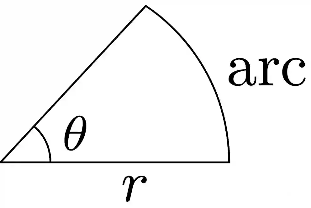
Fig: Plane Angle
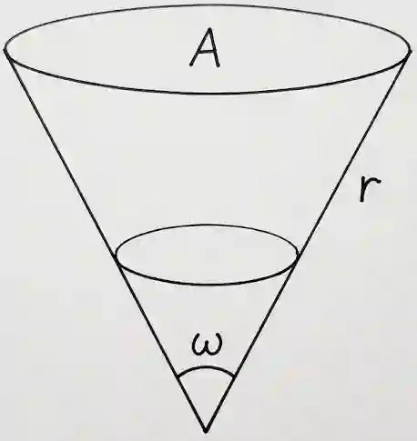
Fig: Solid Angle
Accuracy and Precision
| Accuracy | Precision |
|---|---|
| It is the degree to which the observed value approaches the true value. | It is the degree to which observed values are least scattered. It means how close different measurements are. |
| It is independent of the least count of the measuring equipment. | It depends upon the least count of the measuring equipment. |
| Data is nearer to the true value. | Data are repeated (the range is small). |
For example: A student measured the diameter of a steel ball using a micrometer screw gauge in the lab. The measurements are $6.25 \text{ mm}$, $6.28 \text{ mm}$, $6.23 \text{ mm}$, $6.27 \text{ mm}$, and $6.24 \text{ mm}$. Another student measured the same ball by the same device and measured $6.00 \text{ mm}$, $6.04 \text{ mm}$, $6.12 \text{ mm}$, $6.08 \text{ mm}$, and $6.21 \text{ mm}$. In fact, the correct value is $6.10 \text{ mm}$.
For the 1st Student:
For the 2nd Student:
The 1st student has a smaller range, so his data are more precise. The 2nd student’s average ($6.09 \text{ mm}$) is closer to the accurate value of $6.10 \text{ mm}$, so the 2nd student’s data are more accurate.
• Accuracy = close to the accurate value.
• Precise = less scattered data (i.e., the range of observed data is small).
Uncertainty in Measurement
It is the error in measurement that arises due to the limitations of measuring instruments.
Rules for Rounding Off:
Extra Examples:
Significant Figures (Level of Accuracy)
The numbers of digits in a measurement about which we are reasonably sure are called significant figures.
a) $2000 \text{ m}$ b) $0.2 \times 10^4$ c) $2.0 \times 10^3 \text{ m}$ (Correct answer, because $2.0 \text{ km}$ has 2 SF) d) $2.0 \times 10^2$
Calculation of Significant Figures
The result of addition, subtraction, multiplication, and division of measured values cannot be more accurate than the least accurate measurement.
$$a + b + c = R$$
In addition and subtraction, the final result should be retained to as many decimal places as there are in the number with the least decimal places.
For example: $3.24 + 0.2 = 3.44$ ($\times$ Incorrect) But $3.4$ is the correct answer as there is only one digit after the decimal in $0.2$.
• Mass of box = $1.4 \text{ kg}$ (1 decimal place)
• Mass of ring = $1.32 \text{ gram} = 0.00132 \text{ kg}$ (5 decimal places)
• $1.4 + 0.00132 = 1.40132 \text{ kg}$ But on rounding off to 1 decimal place, we get the result as $1.4 \text{ kg}$.
The final result should retain as many significant figures as there are in the original number with the least significant figures.
For example: $$1.234 \text{ (4 SF)} \times 2.0 \text{ (2 SF)} = 2.468 \text{ (normal multiplication)}$$ $$\rightarrow 2.5 \text{ (multiplication with correct SF)}$$
• $2 \times 5.234 = 10.468$
• $142.06 \text{ (5 SF)} \times 0.23 \text{ (2 SF)} = 32.6728 \text{ (Normal)} \rightarrow$ round off to 2 SF $\rightarrow 33$
Dimensions IMP
Dimensions of physical quantities are defined as the power to which the fundamental units are raised in order to express derived units.
An expression which shows how and which basic units are involved in the derived quantity is called the dimensional formula of that quantity. It is generally written in square brackets [ ].
An equation obtained by equating physical quantities with its dimensional formula is called the dimension equation of that quantity.
| S.N. | Fundamental Quantity | Units | Dimension |
|---|---|---|---|
| 1. | Length | metre (m) | $[L]$ |
| 2. | Mass | kilogram (kg) | $[M]$ |
| 3. | Time | second (s) | $[T]$ |
| 4. | Temperature | kelvin (K) | $[K]$ |
| 5. | Luminosity | candela (cd) | $[J]$ |
| 6. | Electric Current | ampere (A) | $[A]$ |
| 7. | Amount of substance | mole (mol) | $[mol]$ |
Principle of Homogeneity
In every physical relation, the dimension of each term of an equation must be the same.
Solution: $y = a + bx + cx^2$ $y – a – bx – cx^2 = 0$
Now, Dimension of $a$ = Dimension of $y$ $\Rightarrow$ $a = [M^0L^1T^0]$
And, Dimension of $bx$ = Dimension of $y$ $\Rightarrow$ Dimension of $b = \frac{[L]}{[L]} = [M^0L^0T^0]$
And, Dimension of $cx^2$ = Dimension of $y$ $\Rightarrow$ $c [L^2] = [L]$ $\Rightarrow$ $c = \frac{[L]}{[L^2]} = [L^{-1}]$
Therefore, the dimensions of $a, b,$ and $c$ are $[L]$, $[M^0L^0T^0]$, and $[L^{-1}]$ respectively.
Solution: $P = ae^{bt}$ $P – ae^{bt} = 0$
Now, Dimension of $bt = 0$ (exponent/power is dimensionless) $\Rightarrow$ Dimension of $b = \frac{1}{[T]} = [T^{-1}]$
And, Dimension of $ae^{bt}$ = Dimension of $P$ $\Rightarrow$ Dimension of $a = [ML^{-1}T^{-2}]$ (Since $e^{bt}$ is dimensionless, because $e$ is a constant and dimensionless).
Solution: $F – A \cos(Bx) – C \sin(Dt) = 0$
Dimension of $Bx = 0$ $\Rightarrow$ $B = [L^{-1}]$
Dimension of $Dt = 0$ $\Rightarrow$ $D = [T^{-1}]$
(It is because they are dimensionless; $Bx$ and $Dt$ have some numerical value that is dimensionless).
Also, Dimension of $A \cos(Bx)$ = Dimension of $F$ $\Rightarrow$ Dimension of $A = [MLT^{-2}]$ (Since $\cos(Bx)$ gives a dimensionless numeric value).
And, Dimension of $C \sin(Dt)$ = Dimension of $F$ $\Rightarrow$ Dimension of $C = [MLT^{-2}]$ (Same as above).
Now, Dimension of $D/B = \frac{[T^{-1}]}{[L^{-1}]} = [M^0L^1T^{-1}]$
Dimension of $A/C = \frac{[MLT^{-2}]}{[MLT^{-2}]} = [M^0L^0T^0]$
Application of Dimensional Analysis
We will use the principle of homogeneity to check the relation.
Solution: Given: $v^2 = u^2 + 2as$
Dimension of LHS = $[v^2] = [LT^{-1}]^2 = [L^2T^{-2}]$
Dimension of RHS = $[u^2] + [2as] = [LT^{-1}]^2 + [LT^{-2}][L] = [L^2T^{-2}] + [L^2T^{-2}]$
Since Dimension of LHS = Dimension of RHS, the given equation is dimensionally correct.
(a) Escape velocity $v = \sqrt{\frac{2RG}{M}}$ where $R$ and $M$ are Radius and mass of earth respectively and $G$ is the universal gravitational constant.
Solution: Dimension of LHS = $[M^0L^1T^{-1}]$
Dimension of $G = \frac{F \times d^2}{m_1 \cdot m_2} = \frac{[MLT^{-2}] \times [L^2]}{[M^2]} = [M^{-1}L^3T^{-2}]$
Dimension of RHS = $\sqrt{\frac{[L][M^{-1}L^3T^{-2}]}{[M]}} = \sqrt{[M^{-2}L^4T^{-2}]} = [M^{-1}L^2T^{-1}]$
Since $[LHS] \neq [RHS]$, the given equation is dimensionally incorrect.
(b) Time period of Pendulum, $T = 2\pi \sqrt{\frac{l}{g}}$ where $l$ is length and $g$ is acceleration due to gravity.
Solution: Dimension of LHS = $[T]$
Dimension of RHS = $\sqrt{\frac{[L]}{[LT^{-2}]}} = \sqrt{[T^2]} = [T]$
Since $[LHS] = [RHS]$, the given equation is dimensionally correct.
Qn) Derive the dimensional relation of the time period of a pendulum with mass, length, and acceleration due to gravity.
Solution: Let us assume $t \propto m^a l^b g^c$ — (i)
Where: $t = $ time period of pendulum, $l = $ length of pendulum, $m = $ mass of bob, $g = $ acceleration due to gravity
Equation (i) can be written as: $t = k m^a l^b g^c$ (where $k$ is a dimensionless constant)
Writing dimensions on both sides, we get: $[T] = [M]^a [L]^b [LT^{-2}]^c$ $[T] = [M^aL^{b+c}T^{-2c}]$
On equating, we get:
Putting values we get: $t = k m^0 l^{1/2} g^{-1/2}$ $t = k \sqrt{\frac{l}{g}}$
Experimentally: $k = 2\pi$. The required relation is $t = 2\pi\sqrt{\frac{l}{g}}$. It is noted that the time period of a simple pendulum does not depend on the mass of the bob.
Question: Using the method of dimensions, derive an expression for the centripetal force ($F$) acting on a particle of mass ($m$) moving with velocity ($v$) in a circle of radius ($r$).
Let $F \propto m^a v^b r^c$ $F = k m^a v^b r^c$, where $k$ is a dimensionless constant.
Writing the dimensions of LHS and RHS in the equation, we get: $[M L T^{-2}] = k [M]^a [L T^{-1}]^b [L]^c$ $[M L T^{-2}] = k [M^a L^{b+c} T^{-b}]$
Using the principle of homogeneity: $a = 1$, $-b = -2 \implies b = 2$, $b + c = 1 \implies 2 + c = 1 \implies c = -1$
So, the required expression is: $F = k m^1 v^2 r^{-1}$ $\Rightarrow$ $F = \frac{mv^2}{r}$ (where $k=1$)
Converting Units from One System to Another
To convert a unit from one system into another, use the formula:
$$N_1 U_1 = N_2 U_2$$
Solution: The dimension of energy (Joule) is $[M^1 L^2 T^{-2}]$.
| System 1 (SI) | System 2 (New) |
|---|---|
| $N_1 = 10$ | $N_2 = ?$ |
| $M_1 = 1\text{ kg}$ | $M_2 = 100\text{ g}$ |
| $L_1 = 1\text{ m}$ | $L_2 = 10\text{ cm}$ |
| $T_1 = 1\text{ s}$ | $T_2 = 30\text{ s}$ |
We have $N_1 U_1 = N_2 U_2$ $\Rightarrow$ $N_2 = N_1 \left[\frac{U_1}{U_2}\right]$
$N_2 = 10 \times \left[\frac{M_1}{M_2}\right]^1 \left[\frac{L_1}{L_2}\right]^2 \left[\frac{T_1}{T_2}\right]^{-2}$
$N_2 = 10 \times \left[\frac{1\text{ kg}}{100\text{ g}}\right]^1 \left[\frac{1\text{ m}}{10\text{ cm}}\right]^2 \left[\frac{1\text{ s}}{30\text{ s}}\right]^{-2}$
$N_2 = 10 \times \left[\frac{1000\text{ g}}{100\text{ g}}\right] \left[\frac{100\text{ cm}}{10\text{ cm}}\right]^2 [30\text{ s}]^2$
$N_2 = 10 \times 10 \times (10)^2 \times (30)^2$ $\Rightarrow$ $N_2 = 9 \times 10^6$
Therefore, $10 \text{ Joules} = 9 \times 10^6$ new units.
Solution: The dimension of density is $[M L^{-3} T^0]$.
| System 1 (CGS) | System 2 (SI) |
|---|---|
| $n_1 = 11.3$ | $n_2 = ?$ |
| $M_1 = 1\text{ g}$ | $M_2 = 1\text{ kg}$ |
| $L_1 = 1\text{ cm}$ | $L_2 = 1\text{ m}$ |
| $T_1 = 1\text{ s}$ | $T_2 = 1\text{ s}$ |
We have $n_1 U_1 = n_2 U_2$ $\Rightarrow$ $n_2 = n_1 \left[\frac{U_1}{U_2}\right]$
$n_2 = 11.3 \times \left[\frac{M_1}{M_2}\right]^1 \left[\frac{L_1}{L_2}\right]^{-3} \left[\frac{T_1}{T_2}\right]^0$
$n_2 = 11.3 \times \left[\frac{1\text{ g}}{1\text{ kg}}\right]^1 \left[\frac{1\text{ cm}}{1\text{ m}}\right]^{-3} \times 1$
$n_2 = 11.3 \times \left[\frac{1\text{ g}}{1000\text{ g}}\right] \times \left[\frac{1\text{ cm}}{100\text{ cm}}\right]^{-3}$
$n_2 = 11.3 \times 10^{-3} \times (10^{-2})^{-3} = 11.3 \times 10^{-3} \times 10^{+6} = 11.3 \times 10^3$
Value in the SI system = $11.3 \times 10^3\text{ kg/m}^3$.
Solution: Here, $\text{kg/m}^3$ is the unit of density with the dimension $[M^1 L^{-3} T^0]$.
| System 1 (SI) | System 2 (CGS) |
|---|---|
| $n_1 = 5$ | $n_2 = ?$ |
| $M_1 = 1\text{ kg}$ | $M_2 = 1\text{ g}$ |
| $L_1 = 1\text{ m}$ | $L_2 = 1\text{ cm}$ |
| $T_1 = 1\text{ s}$ | $T_2 = 1\text{ s}$ |
Using $n_1 U_1 = n_2 U_2$ $\Rightarrow$ $n_2 = n_1 \times \left[\frac{U_1}{U_2}\right]$
$n_2 = 5 \times \left[\frac{1\text{ kg}}{1\text{ g}}\right]^1 \left[\frac{1\text{ m}}{1\text{ cm}}\right]^{-3} \left[\frac{1\text{ s}}{1\text{ s}}\right]^0$
$n_2 = 5 \times \left[\frac{1000\text{ g}}{1\text{ g}}\right] \left[\frac{100\text{ cm}}{1\text{ cm}}\right]^{-3} \times 1$
$n_2 = 5 \times 1000 \times 1 \times 10^{-6} = 5 \times 10^{-3}$
Therefore, $5\text{ kg/m}^3 = 5 \times 10^{-3}\text{ g/cm}^3$.
Solution: Here, Watt is the SI unit of power. Power ($P$) = $\frac{\text{Work}}{\text{Time}} = [M L^2 T^{-3}]$.
| System 1 (SI) | System 2 (CGS) |
|---|---|
| $n_1 = 10$ | $n_2 = ?$ |
| $M_1 = 1\text{ kg}$ | $M_2 = 1\text{ g}$ |
| $L_1 = 1\text{ m}$ | $L_2 = 1\text{ cm}$ |
| $T_1 = 1\text{ s}$ | $T_2 = 1\text{ s}$ |
We have $n_1 U_1 = n_2 U_2$ $\Rightarrow$ $n_2 = n_1 \times \left[\frac{U_1}{U_2}\right]$
$n_2 = 10 \times \left[\frac{1\text{ kg}}{1\text{ g}}\right]^1 \left[\frac{1\text{ m}}{1\text{ cm}}\right]^2 \left[\frac{1\text{ s}}{1\text{ s}}\right]^{-3}$
$n_2 = 10 \times \left[\frac{1000\text{ g}}{1\text{ g}}\right] \left[\frac{100\text{ cm}}{1\text{ cm}}\right]^2 \times 1$
$n_2 = 10 \times 1000 \times 10000 = 1 \times 10^8$
Therefore, $10\text{ Watts} = 1 \times 10^8\text{ ergs/sec}$.
Finding the Dimension of Constants
Solution: We have $F = \eta A \frac{dv}{dx}$ $\Rightarrow$ $\eta = \frac{F}{A \left(\frac{dv}{dx}\right)}$
Dimension of $F = [M L T^{-2}]$; Dimension of $A = [L^2]$; Dimension of $\frac{dv}{dx} = [T^{-1}]$
Now, by the principle of homogeneity, the dimension of LHS must equal the dimension of RHS. So, the dimension of $\eta$ is:
$$[\eta] = \frac{[M L T^{-2}]}{[L^2][T^{-1}]}$$ $$[\eta] = [M L^{-1} T^{-1}]$$
Limitations of Dimensional Formula
Answer: No, a dimensionally correct equation may not be physically correct. This is because dimensional analysis does not account for constant values. For example, the equations $v = u + at$ and $v = 2u + 3at$ both have the same dimensions $[L T^{-1}]$, but the latter is not physically correct. However, a dimensionally wrong equation is always physically wrong.
📄 View / Download Full PDF Notes
Handwritten Notes
If the PDF doesn’t load, click here to open it in Google Drive.
Typed Notes
If the PDF doesn’t load, click here to open it in Google Drive.
 Physics (भौतिक विज्ञान)
 Chemistry (रसायन विज्ञान)
 Biology (जीव विज्ञान)
 Mathematics (गणित)
 English (अंग्रेजी)
 Nepali (नेपाली)
 Computer Science (कम्प्युटर विज्ञान)
 Account (लेखाशास्त्र)
 Economics (अर्थशास्त्र)
 Business Studies (व्यवसाय अध्ययन)
 Hotel Management (होटल व्यवस्थापन)
 Social (सामाजिक)