
Complete Notes: Slope Stability Analysis
Syllabus Coverage
Unit: Stability of Slopes (4 hours, 6 marks)
2.1 Types of slopes and possible failures
- Natural vs Artificial slopes
- Rotational, Translational failures
- Wedge and Combined failures
2.2 Analysis of infinite slopes
- Dry, submerged conditions
- Seepage parallel to slope
- Critical height calculation
2.3 Analysis of finite slopes
- φu = 0 analysis
- Friction circle method
- Method of slices (Swedish)
2.4 Use of stability charts
- Taylor’s stability number
- Bishop’s method
- Stability coefficients
Table of Contents
- 1. Introduction to Slope Stability
- 2. Factor of Safety (FoS)
- 3. Types of Slope Failure
- 4. Stability Analysis of Infinite Slope
- 5. Finite Slope Analysis
- 6. φu = 0 Analysis (Total Stress)
- 7. Friction Circle Method
- 8. Method of Slices (c-φ Analysis)
- 9. Use of Stability Charts
- 10. Bishop’s Method of Stability Analysis
- 11. Stability Coefficients
- 12. Complete PDF Notes
Introduction to Slope Stability
Slope Stability refers to the potential of soil-covered slopes to withstand and undergo movement. It is a critical aspect in geotechnical engineering for both natural and constructed slopes. The primary goal is to design slopes that are as steep as possible while remaining stable and safe.
Types of Slopes
N
Natural Slopes
These are infinite slopes that extend over large distances with relatively uniform properties.
- Hillsides
- Mountains
- Natural embankments
A
Artificial (Man-made) Slopes
These are finite slopes created by human activity.
Permanent slopes:
- Canals
- Embankments
- Dams
Temporary slopes:
- Excavations
- Trenches
Basic Soil Properties
To analyze stability, basic properties of the soil must be known:
Cohesion (c)
Friction Angle (φ)
Design Principle
A slope should be designed to be as steep as possible while remaining stable and safe. This optimizes construction costs while ensuring safety.
Causes of Slope Failure
Slope failure occurs due to an imbalance between shear strength and shear stress.
Decrease in Shear Strength (s)
Factors reducing strength:
- Weathering: Degradation of soil structure
- Pore Water Pressure: Increase decreases effective stress ($\sigma’ = \sigma – u$)
- Vibrations and Shocks: Disturb soil structure
Increase in Shear Stress (τ)
Factors increasing stress:
- Surcharge: Additional loads on slope top
- Water Content: Increased weight due to saturation
- Seepage Pressure: Forces from flowing water
- Excavation: Geometry changes increase stress
Mobilized Strength
At equilibrium (just before failure), the shear strength mobilized to resist failure is less than maximum available strength.
Mobilized Cohesion
Mobilized Friction Angle
Stability requires: Mobilized stresses < Ultimate strength
Factor of Safety (FoS)
The Factor of Safety ($F$) is defined as the ratio of available strength to the strength required for equilibrium (mobilized strength). Due to uncertainty in soil properties, a higher Factor of Safety is typically chosen to ensure safety.
1. Factor of Safety with respect to Shear Strength ($F_s$)
Where:
$c$ = Cohesion of soil
$\phi$ = Angle of internal friction
$c_m$ = Mobilized cohesion
$\phi_m$ = Mobilized friction angle
For stability, $F$ should be greater than 1.
2. Factor of Safety with respect to Cohesion ($F_c$)
This is the ratio of available cohesion to mobilized cohesion.
3. Factor of Safety with respect to Friction ($F_\phi$)
This is the ratio of the tangent of the friction angle to the tangent of the mobilized friction angle.
Design Criteria
In standard design practice, it is required that the different factors of safety be consistent. Ideally:
Types of Slope Failure
Slope failures are categorized based on the shape of the failure surface and the type of slope.
1. Rotational Failure

Characteristics:
- Occurrence: Takes place in Finite Slopes
- Mechanism: The soil mass slides along a curved surface
- Failure Plane: Circular (slip surface)
- Movement: Downward and outward movement of the soil mass
Varieties:
Toe Failure
The failure surface passes through the toe of the slope
Face Failure
The failure surface passes above the toe (through the slope face)
Base Failure
The failure surface passes below the toe (deep-seated failure)
2. Translational Failure

Characteristics:
- Occurrence: Takes place in Infinite Slopes
- Mechanism: The failure mass slides along a plane parallel to the natural slope ground surface
- Condition: Often occurs when a hard rock layer exists parallel to the slope surface at a shallow depth
3. Other Types of Failure
Combined Failure
- Occurrence: Can happen in Finite Slopes
- Mechanism: A combination of rotational and translational failure mechanisms
Wedge Failure
- Mechanism: Failure takes place along an inclined plane or series of planes (planar failure)
- Shape: The failure mass forms a wedge shape
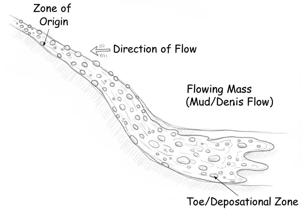
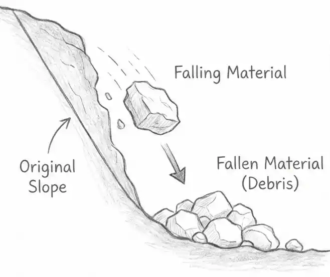
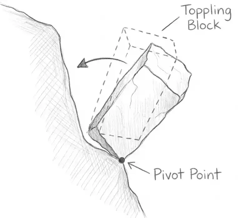
5. Miscellaneous Failure
Includes any failure types other than the four main categories listed above:

Stability Analysis of Infinite Slope
Consider an infinite slope with inclination $i$. We analyze a prismatic element of soil.
Geometry and Forces

Given Parameters:
- Slope Inclination: $i$
- Depth of element: $H$ (vertical depth to failure plane)
- Width of element: $b$ (horizontal width)
- Unit Weight of soil: $\gamma$
Forces acting on the element:
Weight of the Soil Slice ($W$):
(Assuming unit length perpendicular to the page)
Resolving Weight ($W$):
Normal Component ($N$):
Perpendicular to the failure plane
Tangential Component ($T$):
Parallel to the failure plane (driving force)
Stresses on the Failure Plane:
The area of the base of the element along the slope is $A = \frac{b}{\cos i}$ (for unit length).
Normal Stress ($\sigma$):
Shear Stress ($\tau$):
Factor of Safety Formulas for Infinite Slope
1. Cohesionless Soil ($c = 0$)
(a) Dry Soil:
Using dry unit weight $\gamma$:
(b) Submerged Soil:
When the soil is fully submerged, we use the submerged unit weight $\gamma_{sub}$. The ratio of weights cancels out:
(c) Seepage Condition (Steady Seepage Parallel to Slope):
When water flows parallel to the slope surface:
2. Cohesive Soil ($c > 0, \phi > 0$)
(a) Dry Soil:
Using dry unit weight $\gamma$:
(b) Submerged Soil:
Using submerged unit weight $\gamma_{sub}$:
(c) Seepage Condition (Steady Seepage Parallel to Slope):
Using effective stress for strength and saturated weight for driving force:
3. Critical Height ($H_c$)
The critical height is the depth at which failure is imminent ($F = 1$).
Setting $F = 1$ in the cohesive soil equation:
Rearranging to solve for $H_c$:
Finite Slope Analysis
This section covers the stability analysis of finite slopes using various methods for different soil conditions.
Swedish Circle Method (Method of Slices)
This method is used for rotational failure analysis in finite slopes.
Assumptions:
- The failure surface is an arc of a circle with center $O$ and radius $R$
- The soil mass above the failure surface is divided into a number of vertical slices
Procedure:
- Divide the failure mass into vertical slices (strips)
- Consider the forces on a typical slice:
- $W$: Weight of the slice
- $N$: Normal component of weight ($N = W \cos \alpha$)
- $T$: Tangential component of weight ($T = W \sin \alpha$)
- Calculate the resisting and driving moments or forces
Factor of Safety Formula:
Summing forces over all slices:
Where:
- $c \Delta L$: Cohesive force along the base of the slice ($\sum c \Delta L = c \times \text{Length of Arc}$)
- $N \tan \phi$: Frictional resistance
- $T$: Tangential driving force ($W \sin \alpha$)
This assumes the normal force is primarily due to the weight component perpendicular to the arc. This method is the “Fellenius” or “Ordinary Method of Slices”.
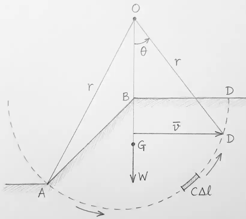
φu = 0 Analysis (Total Stress Analysis)
Figure 5.1 shows a finite slope AB, the stability of which is to be analyzed. Let AD be a trial slip circle, with $r$ as the radius and O as the centre of rotation. Let $\angle AOD = \theta$ and $W$ be the weight of the sliding soil mass ABDA, acting vertically downward through its centre of gravity G, and at a distance $\bar{x}$ from O. The sliding of soil mass ABDA along surface AD amounts to rotation about O.
Moment Analysis:
Taking moments about the centre of rotation O:
Driving moment ($M_D$):
Resisting moment ($M_R$):
where, $l =$ length of arc AD.
Factor of safety against sliding ($F$):
Also, knowing that $\theta = \frac{l}{r}$:
Where:
- $C =$ Cohesion of soil (undrained cohesion $c_u$)
- $W =$ Weight of failure wedge
- $r =$ Radius of slip line
- $\theta =$ Angle in radians
- $\bar{x} =$ Horizontal distance of CG from centre O
Friction Circle Method

The friction circle method assumes the failure surface is cylindrical, i.e., an arc of a circle in section. The sliding mass is assumed to be acted upon by three forces keeping it in equilibrium as shown in Figure 6.1.
Three Forces in Equilibrium:
- The weight ($W$) of the sliding soil mass ABDA, acting vertically through its centre of gravity
- The resultant cohesive force, $C_m \hat{L}$, acting parallel to chord AD and at a distance ‘$a$’ from centre of rotation O.
where, $a = r \cdot \frac{\hat{L}}{\bar{L}}$
$\hat{L} =$ Length of arc AD
$\bar{L} =$ Length of chord AD - The resultant reaction $R$ passing through the point of intersection of the above two forces and tangential to the frictional circle
Procedure:
- Taking centre O and radius $r$, the slip circle AD is drawn. Then, taking centre O and radius $K r \sin \phi$, the frictional circle is drawn. The value of $K$ is taken as unity unless it is specified
- To know the line of action of weight $W$, a vertical line is constructed through the centroid of section ABDA
- Then chord AD is constructed
- To find the line of action of resultant cohesive force $C_m \hat{L}$, a line parallel to chord AD is drawn such that distance $a = r \times \frac{\hat{L}}{\bar{L}}$ from centre O
- Then the length of arc AD, $\hat{L}$, is calculated by using the equation $\hat{L} = \frac{\pi r \delta}{180^\circ}$
- Chord length AD, $\bar{L}$, is found by measurement
- To know the line of action of resultant reaction $R$, a line which is tangential to the frictional circle is constructed from the point of intersection of the line of action of weight $W$ and cohesion force $C_m \hat{L}$
- The weight, $W$, of sliding mass ABDA is calculated and plotted in a suitable scale as shown in Figure 6.1(b). After that, the triangle of forces is drawn in such a way that from the ends of the representing vector $W$, a line is drawn parallel to the lines of action of forces $C_m \hat{L}$ and resultant reaction, $R$
- Then the value of cohesive force $C_m \hat{L}$ is calculated from the force triangle. To find the value of $C_m$, the cohesive force $C_m \hat{L}$ is divided by $\hat{L}$. The factor of safety with respect to cohesion, $F_c$, is given by:
where, $C_m$ is the ultimate cohesionLoading equation…$$F_c = \frac{C}{C_m}$$
Note: A number of slip circles are taken and the factor of safety for each is found. The circle giving the minimum factor of safety is the critical slip circle.
Method of Slices (c-φ Analysis)

The Swedish method of slope stability analysis for c-φ soil is often referred to as the Swedish method of slices. In this analysis, the following assumptions are made:
- The slip surface is cylindrical, i.e., an arc of a circle in section
- The sliding soil mass is assumed to consist of a number of vertical slices
- The forces of interaction between adjacent slices are neglected
Analysis:
Let AD be a slip circle of radius $r$, centre O, and central angle $\angle AOD = \delta$. Let the sliding soil mass ABDA be divided into a number of vertical slices 1, 2, 3… The weights $W_1, W_2, W_3…$ of slices 1, 2, 3… acting through the centre of gravity of the respective slices are resolved into normal components $N_1, N_2, N_3…$ and tangential components $T_1, T_2, T_3…$ as shown in Figure 7.1.
Moment Analysis:
Taking the moment about the centre of rotation O:
Driving moment ($M_D$):
Restoring moment ($M_R$):
Factor of safety against sliding ($F$):
Where:
- $l =$ Length of arc
- $C =$ Cohesion
- $\Sigma T =$ Algebraic sum of tangential components of the weight of slices
- $\Sigma N =$ Algebraic sum of normal components of the weight of slices
A number of trial slip circles are chosen, and the factor of safety of each is computed. The circle which gives the minimum factor of safety is the critical slip circle.
Tabular Calculation Method:
| Slice No. | Width of Slice | Mid-ordinate | Weight of Slice (W) | θ (deg) | N = W cos θ | T = W sin θ |
|---|---|---|---|---|---|---|
| 1 | – | – | $W_1$ | – | $N_1$ | $T_1$ |
| 2 | – | – | $W_2$ | – | $N_2$ | $T_2$ |
| … | … | … | … | … | … | … |
| Σ | $\Sigma N$ | $\Sigma T$ | ||||
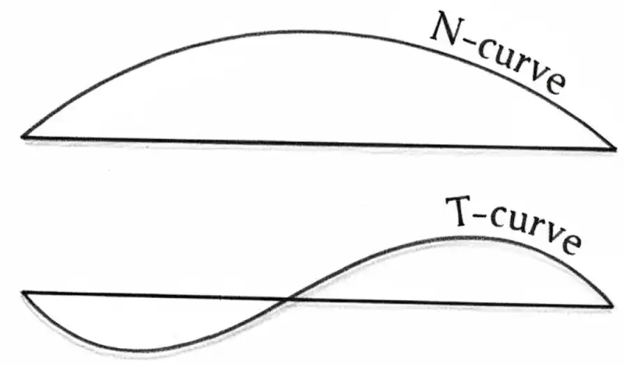
Alternatively, after finding $N_1, N_2 \dots$ and $T_1, T_2 \dots$, N-curves and T-curves can be drawn by plotting N and T values as ordinates for different strips and joining them by smooth curves as shown in Figure 7.2. The areas of these two diagrams are measured using a planimeter to get $\Sigma N$ and $\Sigma T$ values.
Use of Stability Charts – Taylor’s Stability Number
Taylor’s Stability Number ($S_n$)
where,
- $C_m$ = Mobilized cohesion on slip surface
- $\gamma$ = Unit weight of soil
- $H$ = Height of slope
Also, $F_c = \frac{C}{C_m}$ $\therefore$ $C_m = \frac{C}{F_c}$
Further, $F_c = F_H = \frac{H_c}{H}$
where, $H_c$ = critical height of slope
Taylor determined the values of $S_n$ for finite slopes using the friction circle method and presented the result in the form of tables and charts, from which one can obtain the value of $S_n$ for different values of slope angle $i$ and angle of shearing resistance $\phi$.
Taylor also determined the stability number $S_n$ for different values of slope angle $i$ and depth factor $D_f$. The depth factor $D_f$ is defined as:

Taylor’s Stability Tables
Table 1: Taylor Stability Number (Variation with φ and i)
| φ ↓ / i → | 0° | 5° | 10° | 15° | 20° | 25° |
|---|---|---|---|---|---|---|
| 90° | 0.261 | 0.239 | 0.2185 | 0.199 | 0.18 | 0.166 |
| 75° | 0.219 | 0.195 | 0.173 | 0.152 | 0.134 | 0.117 |
| 60° | 0.191 | 0.162 | 0.138 | 0.116 | 0.097 | 0.079 |
| 45° | (0.170) | 0.136 | 0.1085 | 0.083 | 0.062 | 0.044 |
| 30° | (0.156) | (0.110) | 0.075 | 0.046 | 0.0625 | 0.009 |
| 15° | (0.145) | (0.068) | (0.023) | – | – | – |
Table 2: Taylor Stability Number (Variation with Depth Factor $D_f$)
| Slope angle, $i$ | Stability number, $S_n$ | ||||
|---|---|---|---|---|---|
| Depth factor, $D_f$ | 1 | 1.5 | 2 | 3 | ∞ |
| 90° | 0.261 | – | – | – | – |
| 75° | 0.219 | – | – | – | – |
| 60° | 0.191 | – | – | – | – |
| 53° | 0.181 | 0.181 | 0.181 | 0.181 | 0.181 |
| 45° | 0.164 | 0.174 | 0.177 | 0.180 | 0.181 |
| 30° | 0.133 | 0.164 | 0.172 | 0.178 | 0.181 |
| 22.5° | 0.113 | 0.153 | 0.166 | 0.175 | 0.181 |
| 15° | 0.083 | 0.158 | 0.150 | 0.167 | 0.181 |
| 7.5° | 0.054 | 0.080 | 0.107 | 0.140 | 0.181 |
Chart Usage Guidelines:
- For given φ and i, read $S_n$ from chart/table
- Calculate $F_c = \frac{C}{S_n \gamma H}$
- For submerged slopes: Use $\gamma_{sub}$
- For sudden drawdown: Use $\gamma_{sat}$ and weighted φ
Bishop’s Method of Stability Analysis

Assumptions:
- The slip surface is cylindrical, i.e., an arc of a circle in section
- The sliding soil mass is assumed to consist of a number of vertical slices
- The forces of interaction between adjacent slices, which were neglected in the Swedish method, are considered in Bishop’s method
Analysis:
Let AD be a slip circle with radius $r$ and O be the centre of rotation. The section of sliding soil mass ABDA is divided into a number of slices. In Figure 9.1, the free body diagram of a slice between sections $n$ and $n+1$ is shown.
Notations:
- $E_n$ and $E_{n+1}$ = Normal forces on sections $n$ and $n+1$, exerted by adjacent slices
- $X_n$ and $X_{n+1}$ = Shear forces on sections $n$ and $n+1$, exerted by adjacent slices
- $W$ = Weight of slice
- $N$ = Normal reaction at the base of the slice
- $S$ = Shear resistance at the base of slices
- $z$ = Height of slice
- $l$ = Length of the base of slice
- $b$ = Horizontal width of slice
Step-by-step Derivation:
1. Normal stress on base of slice:
2. Effective stress on base of slice:
where, $u$ is the pore pressure
3. Factor of safety against sliding:
4. Shear force on base of slice:
5. Vertical equilibrium of slice:
If $N’$ is the effective normal force; then, $N = N’ + ul$
Substituting the values of $S$ and $N$ in equation (4) and simplifying:
6. Moment equilibrium of entire sliding mass:
Substituting for $S$ and simplifying:
Now, substituting the value of $N’$:
Substituting $x = r \sin \theta$, $b = l \cos \theta$, and assuming $X_n – X_{n+1} = 0$:
Final Bishop’s Equation:
Important Note:
The equation contains the factor of safety $F$ on both sides. The solution has to be obtained by trial and error.
Use of Stability Coefficients (Bishop & Morgenstern Charts)
The equation obtained from Bishop’s method of analysis contains the factor of safety ($F$) on both sides. The solution has to be obtained by trial and error. Hence, to avoid the trial and error solution, Bishop and Morgenstern gave the following expression for the factor of safety:
where $m$ and $n$ are stability coefficients to be obtained from charts prepared by them.
Stability Coefficients:
- The charts give $m$ and $n$ for various values of $\frac{C}{\gamma H}$, depth factor $D_f$, and $r_u$
- The depth factor $D_f$ is defined as:
Loading equation…$$D_f = \frac{\text{Depth of hard stratum below the top of the slope}}{\text{Height of slope}}$$
Hence, the use of stability coefficient is to simplify the analysis.
Comparison of Methods
| Method | Applicability | Assumptions | Accuracy | Complexity |
|---|---|---|---|---|
| φ=0 Analysis | Saturated clays (undrained conditions) | Undrained, φ=0, circular failure surface | Good for short-term analysis | Low |
| Swedish Method (Ordinary Method of Slices) | General c-φ soils | Circular failure, neglects inter-slice forces | Conservative (~10-15% error) | Medium |
| Friction Circle Method | c-φ soils | Total stress, limit equilibrium, circular failure | Moderate | Medium |
| Bishop’s Method | General c-φ soils | Circular failure, considers inter-slice normal forces | Most accurate | High |
| Taylor’s Charts | Preliminary design | Based on friction circle method results | Approximate | Low |
Key Takeaways
Fundamental Concepts
- Slope stability depends on balance between shear strength and shear stress
- Factor of Safety = Available strength / Mobilized strength (F > 1.5 typically)
- Water (seepage) reduces stability significantly (~50% reduction)
- Mobilized strength is less than maximum available strength
Analysis Methods
- Infinite slope formulas depend on soil type and water conditions
- Finite slope analysis methods: φ=0, Swedish slices, Friction circle, Bishop’s
- Taylor’s charts provide quick $S_n$ values for design
- Bishop’s method is most accurate but requires iteration
Failure Types
- Rotational failure (toe, face, base) in finite slopes
- Translational failure in infinite slopes
- Wedge and combined failures
- Miscellaneous failures (flows, falls, topples, slides)
Design Principles
- Design slopes as steep as possible while remaining safe
- Consistent factors of safety: $F = F_s = F_c = F_\phi$
- Consider pore water pressure effects (most critical condition)
- Use appropriate method based on soil type and conditions
Next Topic: Foundation Engineering
Continue to Foundation Engineering Notes